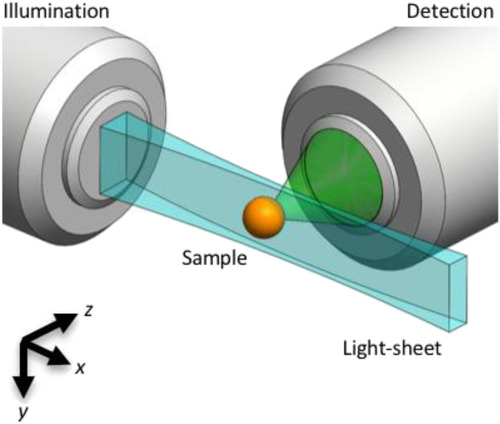
Light-sheet microscopy principle. A light-sheet (blue) can be created by dynamically scanning, along the y direction, a focused Gaussian beam that propagates in the x direction. The focusing is achieved via a low numerical aperture illumination lens. The fluorescence generated by the illuminated (x–y) plane is imaged (green) by an orthogonally positioned wide-field microscope. Axial (x–y) sections of the 3D sample are captured either by scanning the sample (orange) through the stationary focal plane or by scanning the light sheet and detection focal plane through the stationary sample.

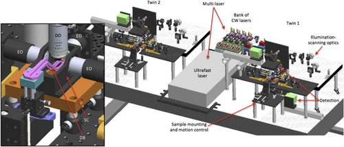
3D opto-mechanical model of the twin-microscope system mounted on a 5 × 10 ft², anti-vibration optical table. Model shows the multi-laser subsystem shared between microscope-twin-1 (right) and microscope-twin-2 (left). Twin-1 has the four functional subsystems labeled and features an implementation of both upright and inverted detection. Brief descriptions of each functional subsystem are provided in Table I. The inset shows a detailed view of the sample chamber (SC), the dive bar (DB) used to hold the sample, three excitation objectives (EO) to deliver excitation light-sheets to the sample, and the detection objective (DO) to collect emitted fluorescence from the sample.

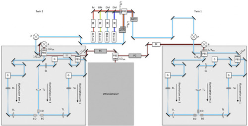
Schematic diagram of multi-laser and illumination-scanning optics subsystems of the instrument. Visible light from the continuous-wave laser bank is fed into microscope-twin 1 (right) and microscope-twin 2 (left) via polarization beamsplitting optics [consisting of a polarizing beamsplitter (PBS) and half-wave plate]. Acousto-optic tunable filters (AOTFs) are used to select the visible wavelengths and adjust the power independently for each twin. The near-infrared (NIR) light from the ultrafast laser is routed similarly using Pockels cells (PCs) to adjust the NIR power independently for each twin. The visible and NIR beams are raised onto 24 × 36 in.² optical breadboards by using periscopes (P). Polarization beamsplitting optics are used both to combine the visible and NIR beams and to split the combined beam into two paths (illumination arms 1 and 2). Illumination arm 1 is further split into two paths through polarization beamsplitting optics, creating a total of three illumination arms. Each illumination arm directs light to the sample through the excitation objectives (EO). BE—beam expander, M—mirror, DM—dichroic mirror, λ/2—half-wave plate, where the subscripts VIS and NIR refer to the visible and near-infrared wavelengths, respectively, G—2D scanning galvo mirrors, SL—scan lens, and TL—tube lens. BE in the NIR twin-2 path appears gray because it is underneath the optical breadboard.

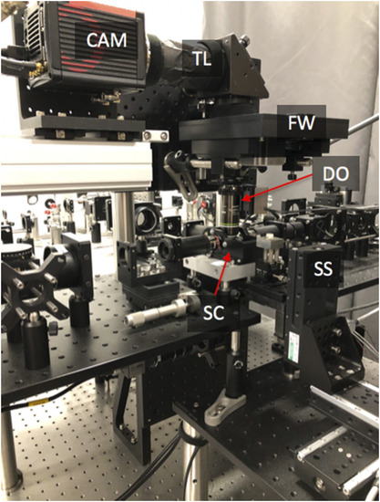
Photograph of an assembled microscope-twin with upright detection. SC—sample chamber, SS—3D stage stack-up, DO—detection objective, FW—filter wheel, TL—tube lens, and CAM—camera.

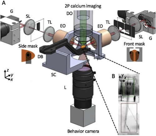
SPIM imaging of intracellular calcium for capturing neuronal activity. (a) Schematic of apparatus for imaging of neural activity during various behaviors in the larval zebrafish. Sheets of laser light are synthesized by quickly scanning the pulsed illumination beam (red) with galvo mirrors (G). 2P light-sheets are delivered to the agarose-embedded head of the animal with excitation objectives (EO) from the side and front arms. The side masks cover each eye on the sides of a horizontally oriented zebrafish, while the front mask covers both eyes, enabling access to neurons between the eyes. 2P-excited calcium fluorescence signal is collected through an upright detection objective (DO) and onto a scientific CMOS camera. A triggerable wide-field camera is positioned below the sample chamber (SC) to provide a wide-field, low-resolution view of the sample, as shown in (b). During a typical neural imaging experiment, the zebrafish larva is mounted in a caddy, which in turn is mounted to the dive bar (DB) underneath the DO. Within the caddy, the zebrafish’s head is immobilized in agarose, while the tail is free, permitting the monitoring of zebrafish behavior through tail movement. SL—scan lens, TL—tube lens, SC—sample chamber, and L—camera lens. The third illumination arm, emission filter, detection TL, scientific camera, light-emitting diode, and filter for behavior channel are not shown. Insets in (b) highlight that the calcium fluorescence channel (green) is recorded from the zebrafish brain, while the behavioral channel (dark red) monitors the tail movement of the animal. Scale bar: (b) 400 µm.

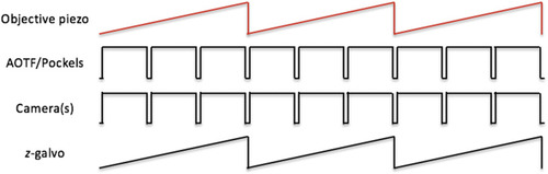
Schematic of control signal sequences for objective-scanning mode. The analog signal representing the position of the objective piezo collar is used as the master timing signal to generate control signals for the imaging cameras (both the fluorescence camera and behavior camera). The timing output of the fluorescence camera controls the AOTF/Pockels. The number of pulses driving the cameras, shown as 3 in the schematic here, determines the number of individual z-plane images to be recorded during a single z-scan cycle over the sample. The position signal of the objective piezo collar, appropriately scaled by a scaling amplifier, is also used to drive the z-galvo.

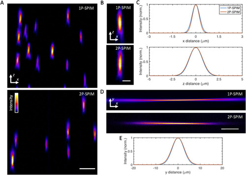
System imaging performance and characterization. (a) y maximum-intensity projections of agarose-embedded 175 nm fluorescent beads imaged at 44× magnification in 1P (top) and 2P excitation mode (bottom). A false-color (fire) lookup table was used to enhance visualization. (b) Selected y maximum-intensity projections of sub-diffraction fluorescent beads in 1P (top) and 2P mode (bottom). (c) Averaged lateral (top) and axial (bottom) full-width at half-maximum (FWHM) extents for the imaged beads, determined by Gaussian fits of 7 bead intensity profiles. The averaged lateral and axial FWHM ±SD values are 1P, 579 ± 15 nm and 1.67 µm± 118 nm, respectively, and 2P, 528 ± 50 nm and 1.78 µm ± 183 nm, respectively. Similar measurements at 11× magnification yield 1P, 1.2 µm ± 86 nm and 1.73 µm ± 387 nm and 2P, 1.17 µm ± 232 nm and 1.81 µm ± 370 nm for lateral and axial directions, respectively. (d) Experimental images of fluorescence excited by 1P (top) and 2P (bottom) Gaussian focused beams, which are scanned in the y direction to create virtual light-sheets. Images were acquired by illuminating a solution of rhodamine in the sample chamber. (e) Intensity line profiles for the focused beams in (d), taken at the center of focus, with approximate FWHM values: 1P, 6.2 µm and 2P, 6.6 µm. These FWHM values yield an averaged light-sheet thickness of ∼10 µm across the 400 µm extent along the x direction, centered around the Gaussian focus. Scale bars: (a) 5 µm, (b) 2.5 µm, and (d) 150 µm.

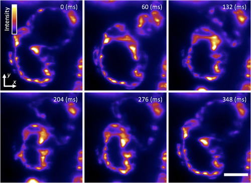
Cardiac light-sheet imaging. Single-plane SPIM recording of the beating heart in a live 5-dpf larval zebrafish with the endocardium fluorescently labeled (GFP), showing six distinct time points during the cardiac beating cycle. These subcellular 2D images are comparable to our previous efforts²¹ as well as recent work by others.³¹ A false-color (fire) lookup table was used to enhance visualization. Frames were captured with a magnification of 11× and 5 ms exposure time at a rate of 85 frames/s. Figure 9 (Multimedia view) shows a movie of the same data. Scale bar: 50 µm.

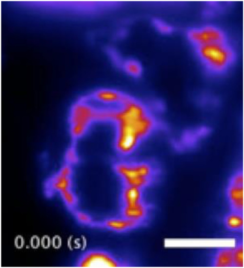
Light-sheet imaging of the dynamic motion of the beating heart of a 5-dpf transgenic larval zebrafish. Same dataset as presented in Fig. 8. Frames were captured at 85 Hz. Scale bar: 50 µm. Multimedia view: https://doi.org/10.1063/1.5144487.110.1063/1.5144487.1

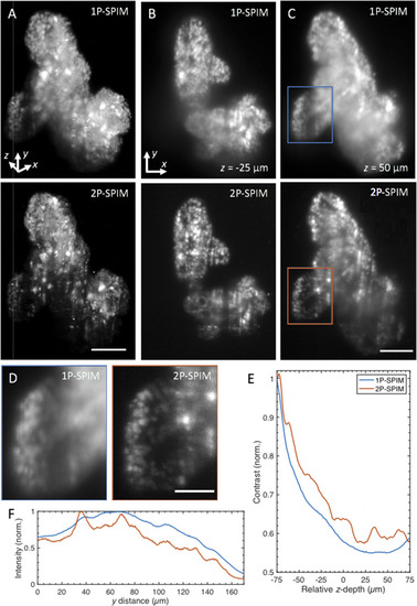
1P- and 2P-SPIM imaging of thick tumor organoids derived from a patient with colorectal cancer. (a) Volume rendering of fixed patient-derived tumor organoids expressing nuclear-localized H2B-GFP recorded in 1P (top) and 2P mode (bottom). Renderings show that the reduced background of 2P-SPIM enables better contrast throughout the imaged volume compared to 1P-SPIM. 3D organoid volume of ∼400 × 550 × 150 (x–y–z) μm³ captured with a magnification of 11×, 1-µm z-steps, and 150 ms exposure time. Figure 11 (Multimedia view) rotates the 3D-rendered volume of the same datasets. (b) and (c) are x–y image slices of (a) at z = −25 µm (50 µm from the surface) and z = 50 µm (125 µm from the surface), respectively. (d) Magnified images of the boxed regions in (c) for 1P (left) and 2P (right) mode revealing that 2P-SPIM resolves more cells than 1P-SPIM deep in the sample. (e) Quantification of image contrast as a function of z-depth. This plot shows quantitatively the improved contrast of 2P-SPIM over 1P-SPIM throughout the imaged volume in (a). Contrast calculated from the standard deviation of the pixel intensities from each x–y image slice and then normalized by the corresponding average image intensity. Each slice (from both modalities) is normalized against the surface slice (z = −75 µm) of 1P-SPIM to show the degradation of performance as a function penetration depth. (f) Plot shows sum intensity along the x direction of images in (d) as a function of light-sheet propagation distance y. The longer NIR wavelength used in 2P-SPIM minimizes the scattering-induced degradation of the excitation light-sheet over longer propagation distances compared to the visible light used in 1P-SPIM. In both intensity profiles, intensity values were normalized by the global maximum. Scale bars: (a) and (c) 100 µm and (d) 50 µm.

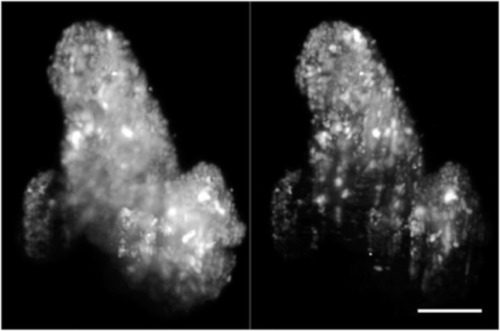
Volume rendering of fixed patient-derived tumor organoids expressing H2B-GFP, comparing images taken with one-photon (1P-, left) and two-photon excitation SPIM (2P-, right). Volumes are rotated around the y and x axes. Same datasets as presented in Fig. 10. Scale bar: 100 µm. Multimedia view: https://doi.org/10.1063/1.5144487.210.1063/1.5144487.2

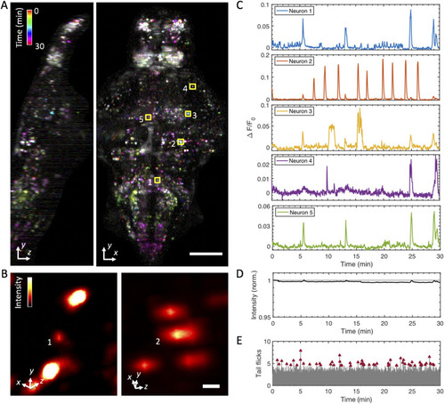
Whole-brain functional imaging at single-cell resolution in behaving 5-dpf transgenic larval zebrafish expressing nuclear-localized calcium indicator elavl3:H2B-GCaMP6s. (a) Maximum-intensity projections of calcium activity are color-coded in time over the 30-min recording window. Active neurons that exhibit fluorescence change during the recording appear as colored dots. Volume of 400 × 800 × 250 (x–y–z) μm³ was sampled by 52 z-planes (4.8 µm z-steps) at 0.5 Hz and 11× magnification. Figure 13 (Multimedia view) shows a 3D rendered movie of the same specimen. (b) Magnified volume renderings of neuron 1 (left) and neuron 2 (right) outlined in the x–y projection in (a), demonstrating cellular resolution in whole-brain 2P-SPIM imaging. The standard deviation projection along the temporal axis was used to generate the renderings, and a false-color (hot) lookup table was used to aid visualization. (c) Representative single-neuron activity traces extracted from the whole-brain recordings, calculated as ∆F/F from the manually selected neurons in (a). (d) Plot shows the total sum intensity of the entire imaged volume as a function of time, normalized to the average intensity of the first 5 min of acquisition (gray line at y = 1). Total intensity exhibits less than a 0.5% decrease in magnitude after the 30-min recording window, indicating that photobleaching is negligible. (e) Analysis of tail flick behavior as a function of time. Tail flicks (movements) obtained by taking the absolute difference in the pixel intensities from the tail region of the wide-field view of the sample, as shown in Fig. 5(b), normalized by the average image intensity corresponding to when there is no tail movement (gray lines). A threshold was applied to classify tail flicks and subsequently confirmed by manual inspection. Tail flicks (red arrowheads), indicating intended swimming behavior, occur throughout the recorded time window (average of ∼9 flicks ±2.2 every 5 min), thus suggesting minimal stress from the imaging conditions used. Scale bars: (a) 100 µm and (b) 5 µm.

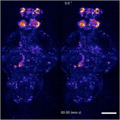
Dorsoventral (left) and rotating (right) maximum-intensity projections of a time-lapse recording of the whole-brain of the a 5-dpf transgenic larval zebrafish. Two-photon whole-brain functional light-sheet imaging was performed at a volumetric rate of 0.5 Hz. The video loops a 5-min recording as part of the data presented in Fig. 12. Scale bar: 100 µm. Multimedia view: https://doi.org/10.1063/1.5144487.310.1063/1.5144487.3