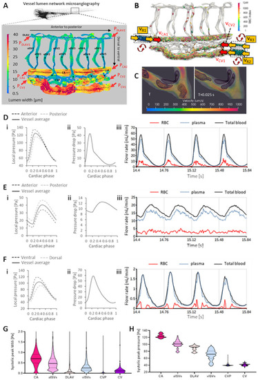
Development of the cell-and-plasma 3-D computational fluid dynamics (CFD) model

(A) Morphology of zebrafish trunk network in the caudal vein plexus region obtained using microangiography and confocal microscopy. Shown are the different vessel types of varying diameter (CA: caudal artery, CV: caudal vein, aISV and vISV: arterial and venous intersegmental vessels, DLAV: dorsal longitudinal anastomotic vessel, CVP: caudal vein plexus). Red arrows indicate the 7 locations where pulsatile pressure input boundary conditions are specified. (B) Red blood cell (RBC) hematocrit in the simulation domain controlled and maintained by recycling cells in the 3 dashed-box domains (RBC indices < 344), see S1 Movie. Yellow arrows indicate reservoir velocity periodic boundary inputs copied from the adjacent region (red arrow) in the trunk network. (C) Collision of RBCs with vessel walls and with one another as part of the explicit consideration of blood dynamics in the CFD model (S2 Movie). (D and E) Pulsatile pressure boundary conditions defined at the anterior and posterior ends of the CA (Di) and CV (Ei) and the resulting pulsatile pressure drop across the CA (Dii) and CV (Eii) that drives the pulsatile flow of RBC and plasma blood phases in the CA (Diii) and CV (Eii). (F) Pulsatile pressures arising at the dorsal and ventral ends of aISV3 (i) due to oscillating pressure inputs at anterior and posterior ends of the CA and CV, and the resulting pulsatile pressure drop across aISV3 (ii) that drives the pulsatile flow of RBC and plasma blood phases in aISV3 (iii). (G and H) Hierarchical stratification of WSS (G) and blood pressure (H) levels in the network predicted by CFD; see S1 Movie for spatial maps of oscillating WSS and pressure.

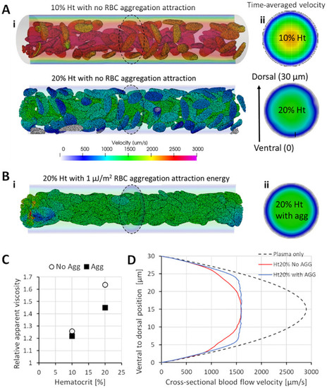
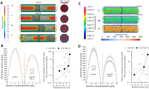
Effects of RBC hematocrit and aggregation on viscosity and blood flow velocity.

(A) Snapshots of RBC arrangement and velocity driven by steady state 9.6 Pa pressure drop from left to right ends of the vessel segment (30 μm in diameter and 150 μm in length) under 10 and 20% hematocrits (i) and the time-averaged blood velocity plot in the cross-sectional lumen at the middle of the vessel length (ii). (B) Snapshots of RBC rouleaux formation and velocity under 20% hematocrits and 1 μJ/m² aggregation levels (i) and the time-averaged blood velocity plot in the cross-sectional lumen at the middle of the vessel length (ii). (C) Plot of relative apparent viscosity against hematocrit for blood with and without RBC aggregation. Movies of the four conditions simulated can be viewed in S3–S5 Movies. (D) Flow retardation effect of RBCs in blood flow and the flow blunting effects of RBC aggregation on the cross-sectional velocity profile under constant segment pressure drop conditions.

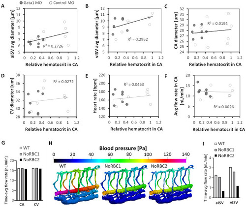
Systemic alteration in vessel morphology and blood flow in zebrafish with reduced RBC hematocrit.

(A to D) Diameters of aISV: p = 0.046 (A), vISV: p = 0.036 (B), CA: p = 0.63 (C) and CV: p = 0.56 (D) as functions of the relative CA hematocrit in gata1 and control morphants. (E to F) Heart rate: p = 0.44 (E) and estimated flow rate: p = 0.86 (F) as functions of the relative CA hematocrit. Statistical significances of slopes in A to F were determined using regression t-test. (G) CFD model predictions of blood flow rates in CA (16.15, 16.15, 15.76 nL/min) and CV (16.21, 16.34, 16.06 nL/min) for WT (14% Ht), NoRBC1 (0% Ht) and NoRBC2 (0% Ht and 18% ISV diameter reduction). (H) CFD predictions of systolic pressure distribution maps in models WT, NoRBC1 and NoRBC2. (I) CFD predicted blood flow rates in the aISVs (-9.1% and -70% for NoRBC1 and NoRBC2, respectively, compared to WT) and vISVs (-15% and -61% for NoRBC1 and NoRBC2, respectively, compared to WT).

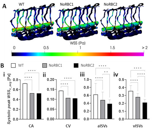
Decrease in ISV diameter exacerbates the decrease in WSS caused by hematocrit reduction.

(A) Systolic WSS distributions in models WT (14% Ht), NoRBC1 (0% Ht) and NoRBC2 (0% Ht and 18% ISV diameter reduction). (B) Predicted systolic WSS levels in the CA (i), CV (ii), aISVs (iii) and vISVs (iv) for the 3 models. Statistical comparisons were performed using one-way ANOVA with Sidak’s multiple pair comparisons. **, p < 0.01; ****, p < 0.0001.

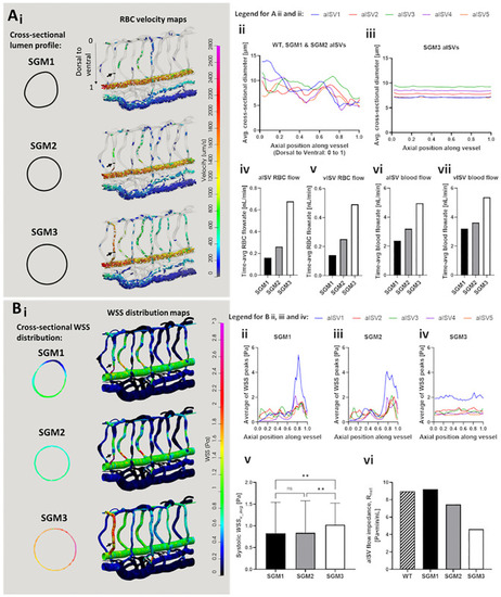
Simulation predictions of flow and WSS distribution in networks with ISVs of varying diameters and cross-sectional shapes.

(see also S6 Movie). (A) RBC partitioning and velocity maps for the 3 SGM networks. Magnified cross-sectional profile of aISV1 lumen at 0.75 dorsal-to-ventral position is indicated for the 3 SGM by the arrows (Ai). The variation in average cross sectional aISV lumen diameter along the dorsal-to-ventral axis observed for WT network that was similarly prescribed in the SGM1 and SGM2 ISVs (Aii). The geometric averaging of lumen diameter applied across ISV axis in the SGM3 network (Aiii). Time-averaged aISV (Aiv) and vISV (Av) RBC flow rates. aISV (Avi) and vISV (Avii) blood flow rates across the 5 aISVs in the SGM models. (B) Systolic peak WSS maps for the 3 SGM networks and the magnified cross-sectional WSS distribution in aISV1 lumen at 0.75 dorsal-to-ventral position (Bi). Dorsal-to-ventral plots of systolic WSS in aISVs in the SGM1 (Bii), SGM2 (Biii) and SGM3 (Biv) networks. Comparison of the average systolic WSS (Bv) and the corresponding vessel flow impedance (R_net) (Bvi) across the 5 aISVs in the 3 SGM networks. Statistical comparisons were performed using one-way ANOVA with Sidak’s multiple pair comparisons. **, p < 0.01.

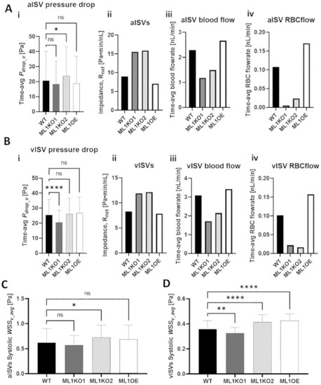
Hemodynamics adaptation scenarios for Marcksl1 OE and Marcksl1 KO.

(A) WT levels of RBC (i) and systolic blood pressure (ii) distribution, see S1 Movie. (B) Marcksl1 OE model (ML1OE) with same blood pressure boundary conditions (BCs) at anterior/posterior input locations as WT. Spatial maps of RBC perfusion (Bi) and systolic blood pressure distribution (Bii) where yellow dashed circles indicate the locally dilated lumen region compared to WT (Bi), see S7 Movie. Dashed red box region in Aii and Bii is the local network region where pressure distribution has been altered between WT and ML1OE. (C—E) Marcksl1 KO Model 1 (ML1KO1, C) with reduced blood pressure BCs, Marcksl1 KO Model 2 (ML1KO2, D) with same blood pressure BCs as WT and Marcksl1 KO Model 3 (ML1KO3, E) with increased blood pressure BCs. Spatial maps of RBC perfusion (i) and systolic blood pressure distribution (ii), see S8–S10 Movies.

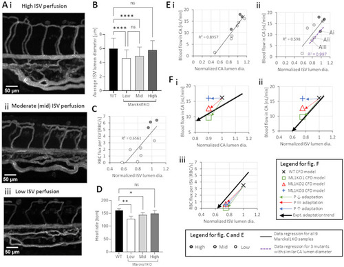
Characterization of RBC flow in Marcksl1 KO zebrafish with reduced vessel diameters.

(A) Representative maximum intensity time-stack projection images of RBC flow in the ISV networks of 2 dpf Marcksl1 KO zebrafish, from high (i), moderate/mid (ii) to low (iii) perfusion. (B) Comparison of average ISV lumen diameters of Marcksl1 KO zebrafish in different perfusion level groups versus WT. (C) RBC flux reduction in ISVs in response to ISV lumen diameter reduction (in Marcksl1 KO zebrafish). (D) Comparison of heart rate in Marcksl1 KO zebrafish versus WT. Statistical comparisons in B and D were performed using one-way ANOVA with Sidak’s multiple pair comparisons. *, p < 0.05; **, p < 0.01; ****, p < 0.0001. (E) Experimental observations of flow reductions in Marcksl1 KO mutants. Arterial blood flow reduction in CA in response to reduced CA lumen diameters (i). Arterial blood flow reduction in CA in response to reduced ISV lumen diameters (ii). Purple dashed lines indicate data points from the same embryos in Ai to Aiii, which have similar CA lumen diameter. (F) Comparison between the modeled adaptation scenarios (green, red and blue arrows) compared to experimentally observed adaptation trends (black arrow: regression data from E) for CA blood flow against CA diameter (i), CA blood flow against ISV lumen diameter (ii) and RBC flux entering ISVs against ISV lumen diameter (iii).

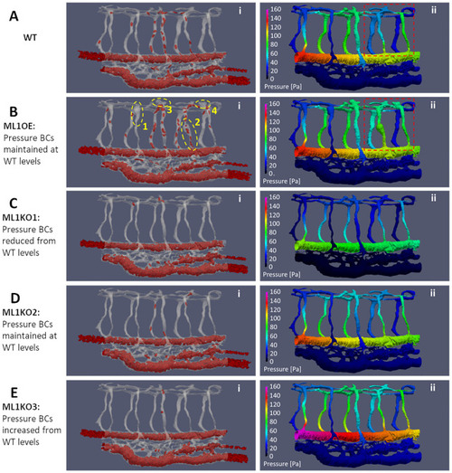
Comparison of pressure and WSS distributions in ISVs amongst WT and Marcksl1 network models.

(A) Group-average (5 aISVs) of the time-averaged pressure drop (P_{drop_v}) in aISVs amongst models (i) and the corresponding impedance (R_net) (ii), blood flow rate (iii) and RBC flow rate (iv) in the aISVs. (B) Group-average (5 vISVs) of the time-averaged pressure drop (P_{drop_v}) in vISVs amongst models (i) and the corresponding R_net (ii), blood flow rate (iii) and RBC flow rate (iv) in the vISVs. (C) Group-averaged (5 aISVs) systolic peak WSS (WSS_{v_avg}) in aISVs amongst models. (D) Group-averaged WSS_{v_avg} in vISVs amongst models. Statistical comparisons were performed using one-way ANOVA with Sidak’s multiple pair comparisons. *, p < 0.05; **, p < 0.01; ****, p < 0.0001.

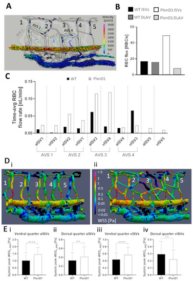
Hemodynamic alterations arising from network mispatterning in PlxnD1 model

(see S11 Movie). (A) Spatial distribution map of RBC trajectories/velocities at systolic peak. Dashed lines indicate arterial-venous shunts that bypass DLAV connections in the ISV network. (B) The flux bypass in ISV-DLAV network in PlxnD1 versus the ISV-DLAV network in WT. (C) Comparison of the time-averaged RBC flow rate in ISVs between WT and PlxnD1 models. (D) WSS spatial distribution map in WT (Di) and PlxnD1 (Dii) network models. Red bold lines in Dii indicate low-WSS dead flow regions. (E) Comparison of the ventral (i) and dorsal (ii) levels of systolic peak WSS between WT and PlxnD1 aISVs, the ventral (iii) and dorsal (iv) levels of systolic peak WSS between WT and PlxnD1 vISVs. Statistical comparisons in E and F were performed using unpaired two-tailed t test. **, p < 0.01; ****, p < 0.0001.

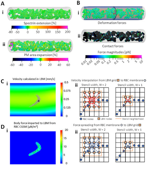
The fundamental components and physics of the cell-and-plasma phase CFD model.

(A) Membrane deformation characteristics modelled by the coarse-grained spectrin model (CGSM) in terms of spectrin extension (i) and plasma membrane areal expansion (ii). (B) Forces arising in the CGSM due to membrane deformations (i) and cell-cell & cell-lumen-wall contact (ii). (C) Schematics of the velocity update in the immersed boundary method (IBM) where surrounding fluid velocities calculated by the lattice Boltzmann method (LBM) solver (i) are interpolated to membrane point in accordance with Eqs (7) & (8) and the stencil width W (ii). (D) Schematics of the momentum update in the immersed boundary method where forces of deformation in the membrane (solved by CGSM) are spread to the fluid as body-forces (i) in accordance with Eqs (8) & (9) and the stencil width W (ii).

Grid independence testing for numerical accuracy and precision in the simulations.

(A) Snapshots of the ISV-domain grid testing simulations with an 8 μm diameter by 40 μm length vessel segment under steady-state 18 Pa flow-driving pressure. The simulations were performed with computational grids at very fine (VF), fine (F), medium (M) and coarse (C) grid resolutions. For clarification of the grid resolution dimensions refer to main text. Plot fills are colored for flow velocity on the left image while circle cross sections on the right image indicate the grid voxels which are colored in red for lumen and blue for vessel wall. (B) The predicted flow velocities under varying grid resolutions (left) and the computing-cost versus simulation error matrix (right). (C) Snapshots of the CA-domain grid testing simulations with a 30 μm diameter by 150 μm length vessel segment under steady-state 18 Pa flow-driving pressure. The simulations were performed with computational grids at fine (F), medium (M) and coarse (C) grid resolutions. Plot fills are colored for flow velocity on the left image. (D) The predicted flow velocities under varying grid resolutions (left) and the computing-cost versus simulation error matrix (right).