
- Title
-
Activity regulates a cell type-specific mitochondrial phenotype in zebrafish lateral line hair cells
- Authors
- McQuate, A., Knecht, S., Raible, D.W.
- Source
- Full text @ Elife
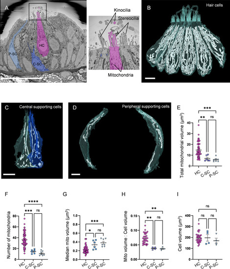
(A) SEM cross-section through 5 days post fertilization (dpf) zebrafish neuromasts (NM) (NM3, Figure 1—source data 2). Scale bar = 20 µm. Inset shows the stereocilia bundle and kinocilium labeled for 1 HC. (B) Six reconstructed HCs from NM3, with mitochondria shown in white. Scale bar = 5 µm. (C) Two central supporting cells (C-SCs) reconstructed from NM3. Scale bar = 5 µm. (D) Two peripheral supporting cells (P-SCs) reconstructed from NM3. Scale bar = 3.5 µm. (E) Sum of mitochondrial volume for HCs, C-SCs, and P-SCs. (In µm3) HC: 14.8 ± 0.8; C-SC; 6.9 ± 1.1, P-SC; 6.0 ± 0.7. (F) Number of individual mitochondria in HCs, C-SCs, and P-SCs. HC: 36.1 ± 1.6; C-SC: 14.5 ± 1.4; P-SC: 10.9 ± 1.5. (G) The median mitochondrial volume in HCs, C-SCs, and P-SCs. HC: 0.2 ± 0.01; C-SC: 0.3 ± 0.04; P-SC: 0.4 ± 0.03. (H) The ratio of the total mitochondrial volume to the total cell volume in HCs, C-SCs, and P-SCs. HC: 0.07 ± 0.003; C-SC: 0.04 ± 0.002; P-SC: 0.04 ± 0.002. (I) The cell volume of HCs, C-SCs, and P-SCs. HC: 195.6 ± 7.2; C-SC: 197.4 ± 30.05; P-SC: 170.4 ± 22.7. Kruskal–Wallis test with Dunn’s multiple comparisons, *p<0.05, **p<0.01, ***p<0.001, ****p<0.0001. For (E–G), HC: n = 65, 5 NMs, 3 fish; C-SC: n = 6, 3 NMs, 2 fish; P-SC: n = 7, 3 NMs, 2 fish. For (H, I), HCs: n = 35, 3 NMs, 3 fish; C-SC: n = 4, 2 NMs, 2 fish; P-SC: n = 4, 2 NMs, 2 fish. Data are presented as the mean ± SEM.
|
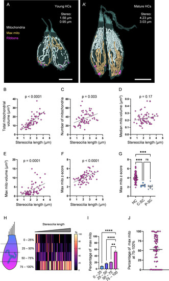
(A) Two young HCs from a 5 days post fertilization (dpf) neuromasts (NM) (NM1, Figure 2—source data 2). Mitochondria are shown in white. Single largest mitochondrion (max mito) is shown in gold. Synaptic ribbons shown in purple. Scale bar = 5 µm. (A’) Two mature HCs from a 5 dpf NM (NM3, different HCs than in Figure 1B). Scale bar = 6 µm. (B) Relationship between HC stereocilia length and the total mitochondrial volume. (C) Relationship between HC stereocilia length and the number of individual mitochondria. (D) Relationship between HC stereocilia length and the volume of the median mitochondrion. (E) Relationship between HC stereocilia length and the volume of the largest mitochondrion (max mito). (F) Relationship between HC stereocilia length and the number of standard deviations between the max mito and average mitochondrial volume (max mito z-score). Lines represent standard linear regression, with significance as indicated. (G) The z-score of the max mito in HCs, central supporting cells (C-SCs), and peripheral supporting cells (P-SCs) (mean ± SEM) HC: 4.1 ± 0.1; C-SC: 2.4 ± 0.1, P-SC: 2.1 ± 0.2. Kruskal–Wallis test with Dunn’s multiple comparisons, ***p<0.001. (H) The percentage of the max mito located within each quadrant of an HC represented as a heat map. The length of each HC was normalized and broken into quadrants, with the highest HC point the base of the stereocilia bundle and the lowest point the lowest ribbon. The number of max mito segmentation coordinates within each quadrant of an HC were counted and represented as a percentage of all max mito coordinates. Cells are presented in order of their stereocilia lengths. (I) Summary of heat map data shown in (H). Most apical quadrant (0–25%): 9 ± 2.4%; 25–50%: 17.1 ± 2.7%; 50–75%: 21 ± 2.2%; Most basal quadrant (75–100%): 52.8 ± 4.4%. Kruskal–Wallis test with Dunn’s multiple comparisons, **p<0.01, ****p<0.0001. (J) Percentage of the max mito located within the most basal quadrant for individual HCs. HC: n = 65, 5 NMs, 3 fish; C-SC: n = 6, 3 NMs, 2 fish; P-SC: n = 7, 3 NMs, 2 fish.
|
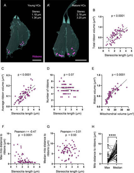
(A) Two representative young hair cells (HCs) from a 6 days post fertilization (dpf) neuromasts (NM) (NM4, Figure 3—source data 2) with synaptic ribbons shown in purple. Scale bar = 4.5 µm. (A’) Two representative mature HCs from a 6 dpf NM (NM4, Figure 3—source data 2). Scale bar = 4 µm. (B) Relationship between HC stereocilia length and the total ribbon volume. (C) Relationship between HC stereocilia length and the average ribbon volume. (D) Relationship between HC stereocilia length and the number of ribbons. (E) Relationship between HC total mitochondrial volume and HC ribbon volume. Black line = standard linear regression, with significance as indicated. (F) Relationship between HC stereocilia length and the average minimum distance between each ribbon and the max mito. (G) Relationship between HC stereocilia length and the average minimum distance between each ribbon and the median mito. (H) Average minimum distance between each ribbon and the HC max or median mito. (In µm) Max mito: 1.9 ± 0.3; median mito: 6.3 ± 0.3. Mann–Whitney test, ****p<0.0001. HC: n = 65, 5 NMs, 3 fish, 5–6 dpf.
|
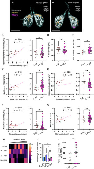
(A) Representative young HCs from a 3 dpf neuromasts (NM) (NM6, Figure 4—source data 2). Max mito shown in gold. Synaptic ribbons shown in purple. Scale bar = 8 µm. (A’) Representative older HCs from a 3 dpf NM (NM6, Figure 4—source data 2). Scale bar = 6 µm. (B) Comparison of total mitochondrial volume development (left) and average (right) between 3 dpf and 5–6 dpf HCs. On average (in µm3): 3 dpf: 14.4 ± 1.2; 5–6 dpf: 14.8 ± 0.8. Kolmogorov–Smirnov test, p=0.49. (C) Total HC volume for 3 dpf and 5–6 dpf HCs. (In µm3) 3 dpf: 210.1 ± 11.3; 5–6 dpf: 195.6 ± 7.2. Kolmogorov–Smirnov test, p=0.2. (C’) Ratio of total mitochondrial volume to HC volume. 3 dpf: 0.06 ± 0.003; 5–6 dpf: 0.07 ± 0.003. Kolmogorov–Smirnov test, p=0.41. (D) Comparison of the number of HC mitochondria over development (left) and on average (right) in 3 dpf and 5–6 dpf HCs. On average: 3 dpf: 25.0 ± 2; 5–6 dpf: 36.1 ± 1.6. Kolmogorov–Smirnov test, p=0.022. (E) Comparison of the median mitochondrial volume over development (left) and on average (right). On average (in µm3): 3 dpf: 0.3 ± 0.02; 5–6 dpf: 0.2 ± 0.01. Kolmogorov–Smirnov test, p=0.005. (F) Comparison of the max mito volume over development (left) and on average (right). On average (in µm3): 3 dpf: 3.8 ± 0.5; 5–6 dpf: 3.5 ± 0.4. Kolmogorov–Smirnov test, p=0.32. (G) Comparison of the max mito z-score in 3 dpf and 5–6 dpf HCs over development (left) and on average (right). On average: 3 dpf: 3.7 ± 0.3; 5–6 dpf: 4.1 ± 0.1. Standard unpaired t-test, p=0.21. (B–G) Solid line represents the standard linear regression for 3 dpf HCs. Dashed line represents standard regression for the 5–6 dpf HCs dataset as in Figure 2. Significance of the 3 dpf regression and difference with 5–6 dpf regression slope (S) are indicated. (H) The percentage of the max mito located within each quadrant of 3 dpf HCs represented as a heat map. Two HCs in the 3 dpf dataset lacked ribbons to provide a consistent HC lowest point and were not included in this analysis. (I) Summary of the heat map data shown in (H). Most apical quadrant (0–25%): 24.9 ± 8.9%; 25–50%: 37.2 ± 5.7%; 50–75%: 16.0 ± 4.2%; Most basal quadrant (75–100%): 22.0 ± 7.9%. Kruskal–Wallis test with Dunn’s multiple comparisons, nonsignificant. (J) Percentage of max mito located within the most basal quadrant for individual HCs. 3 dpf: 22.0 ± 7.9%, 5–6 dpf: 52.8 ± 4.4%. Kolmogorov–Smirnov test, p=0.017. Same cells as in (H, I). (B, D–G) 3 dpf data: n = 12 HCs, 2 NMs, 2 fish. 5–6 dpf data: n = 65 HCs, 5 NMs, 3 fish. (C, C’) 3 dpf data: n = 12 HCs, 2 NMs, 2 fish. 5–6 dpf data: n = 35 HCs, 3 NMs, 3 fish. (H–J) 3 dpf data: n = 10 HCs, 2 NMs, 2 fish. 5–6 dpf data: n = 65 HCs, 5 NMs, 3 fish. Where applicable, data are presented as the mean ± SEM.
|
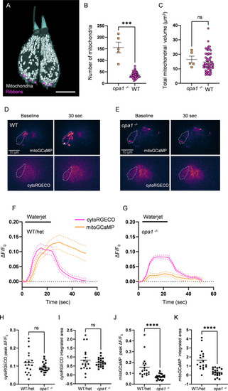
(A) Two representative opa1 HCs (Figure 5—source data 2). Scale bar = 5 µm. (B) Number of individual mitochondria in WT and opa1 HCs. WT: 36.1 ± 1.6; opa1: 155.6 ± 23.22. Kolmogorov–Smirnov test, p=0.0002. (C) Total mitochondrial volume in WT and opa1 HCs. In µm3, WT: 14.8 ± 0.8; opa1: 16.5 ± 2.3. Kolmogorov–Smirnov test, p=0.66. (B, C) opa1 HCs; n = 5 HCs, 1 NM, 1 fish. (D) Representative WT images of myo6:mitoGCaMP (top) and myo6:cytoRGECO (bottom) at baseline and following a waterjet stimulus. (E) Same as in (D), but for opa1 HCs. (F, G) Changes in myo6:mitoGCaMP and myo6:cytoRGECO Ca2+ signal (expressed as ΔF/F0) following a 20 s, 10 Hz waterjet for both WT/het (F) and opa1 HCs (G). (H) Peak myo6:cytoRGECO ΔF/F0 signal. WT/het: 0.1 ± 0.02; opa1: 0.1 ± 0.01, Mann–Whitney test, p=0.28. (I) Integrated myo6:cytoRGECO ΔF/F0 signal. WT/het: 0.8 ± 0.2; opa1: 0.7 ± 0.05, Mann–Whitney test, p=0.94. (J) Peak myo6:mitoGCaMP ΔF/F0 signal. WT/het: 0.15 ± 0.02; opa1: 0.05 ± 0.007, Mann–Whitney test, p<0.0001. (K) Integrated myo6:mitoGCaMP ΔF/F0 signal. WT/het: 1.6 ± 0.3; opa1: 0.2 ± 0.1, Mann–Whitney test, p<0.0001. (D–K) WT/het: n = 18 HCs, 7 fish. opa1: n = 20 HCs, 9 fish. Data are presented as the mean ± SEM.
|
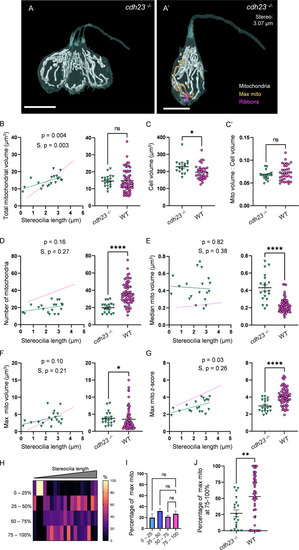
(A) Three representative cdh23 hair cells (HCs) with mitochondria labeled in white (from NM11, Figure 6—source data 2). Scale bar = 9.5 µm. (A’) Representative mature cdh23 HC (NM11), max mito shown in gold, synaptic ribbons shown in purple. Scale bar = 6 µm. (B) Comparison of total mitochondrial volume development (left) and average (right) between cdh23 and WT HCs. On average (in µm3): cdh23:14.6 ± 0.8; WT: 14.8 ± 0.8. Kolmogorov–Smirnov test, p=0.35 (C) Total HC volume for cdh23 and WT HCs. (In µm3) cdh23: 228.0 ± 10.3; WT: 195.6 ± 7.2. Kolmogorov–Smirnov test, p=0.03. (C’) Ratio of total mitochondrial volume to HC volume. cdh23: 0.07 ± 0.002; WT: 0.07 ± 0.003. Kolmogorov–Smirnov test, p=0.23. (D) Comparison of the number of HC mitochondria over development (left) and on average (right) in cdh23 and WT HCs. On average: cdh23: 19.8 ± 1.4; WT: 36.1 ± 1.6. Kolmogorov–Smirnov test, p<0.0001. (E) Comparison of the median mitochondrial volume over development (left) and on average (right). On average (in µm3): cdh23: 0.4 ± 0.04; WT: 0.2 ± 0.01. Kolmogorov–Smirnov test, p<0.0001. (F) Comparison of the max mito volume over development (left) and on average (right). On average (in µm3): cdh23: 3.8 ± 0.5; WT: 3.5 ± 0.4. Kolmogorov–Smirnov test, p=0.04. (G) Comparison of the max mito z-score in cdh23 and WT HCs over development (left) and on average (right). On average: cdh23: 3.0 ± 0.2; WT: 4.1 ± 0.1. Standard unpaired t-test, p<0.0001. (B–G) Solid line represents the standard linear regression for cdh23 HCs. Dashed line represents standard regression for WT HCs as in Figure 2. Significance of the cdh23 regression and differences in the slope from the WT regression (S) are indicated. (H) The percentage of the max mito located within each quadrant of cdh23 HCs represented as a heat map. (I) Summary of the heat map data shown in (H). Most apical quadrant (0–25%): 19.8 ± 7.0%; 25–50%: 31.9 ± 4.8%; 50–75%: 21.6 ± 2.6%; Most basal quadrant (75–100%): 26.8 ± 5.3%. Kruskal–Wallis test with Dunn’s multiple comparisons, nonsignificant. (J) Percentage of max mito located within the most basal quadrant for individual HCs. cdh23: 26.8 ± 5.3%, WT: 52.8 ± 4.4%. Kolmogorov–Smirnov test, p=0.008. (B, D–J) cdh23 data: n = 19 HCs, 4 NMs, 2 fish. WT data: n = 65 HCs, 5 NMs, 3 fish. (C, C’) cdh23 data: n = 17 HCs, 4 NMs, 2 fish. WT data: n = 35 HCs, 3 NMs, 3 fish. Where applicable, data are presented as the mean ± SEM.
|
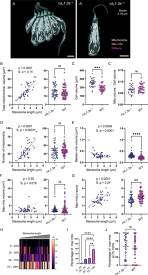
(A) Six representative cav1.3a hair cells (HCs) with mitochondria labeled in white (from NM13, Figure 7—source data 2). Scale bar = 5 µm. (A’) Representative mature cav1.3a HC (NM14, Figure 7—source data 2), max mito shown in gold, synaptic ribbons shown in purple. Scale bar = 5 µm. (B) Comparison of total mitochondrial volume development (left) and average (right) between cav1.3a and WT HCs. On average (in µm3): cav1.3a: 16.2 ± 1.0; WT: 14.8 ± 0.8. Kolmogorov–Smirnov test, p=0.76. (C) Total HC volume for cav1.3a and WT HCs. (In µm3) cav1.3a: 252.5 ± 9.3; WT: 195.6 ± 7.2. Kolmogorov–Smirnov test, p=0.0003. (C’) Ratio of total mitochondrial volume to HC volume. cav1.3a: 0.07 ± 0.003; WT: 0.07 ± 0.003. Kolmogorov–Smirnov test, p=0.66. (D) Comparison of the number of HC mitochondria over development (left) and on average (right) in cav1.3a and WT HCs. On average: cav1.3a: 34.9 ± 3.0; WT: 36.1 ± 1.6. Kolmogorov–Smirnov test, p=0.13. (E) Comparison of the median mitochondrial volume over development (left) and on average (right). On average (in µm3): cav1.3a: 0.3 ± 0.02; WT: 0.2 ± 0.01. Kolmogorov–Smirnov test, p<0.0001. (F) Comparison of the max mito volume over development (left) and on average (right). On average (in µm3): cav1.3a: 2.6 ± 0.2; WT: 3.5 ± 0.4. Kolmogorov–Smirnov test, p=0.14. (G) Comparison of the max mito z-score in cav1.3a and WT HCs over development (left) and on average (right). On average: cav1.3a: 3.4 ± 0.1; WT: 4.1 ± 0.1. Standard unpaired t-test, p=0.001. (B–G) Solid line represents the standard linear regression for cav1.3a HCs. Dashed line represents standard regression for WT HCs dataset as in Figure 2. Significance of the cav1.3a regression and differences in the slope from the WT regression (S) are indicated. (H) The percentage of the max mito located within each quadrant of cav1.3a HCs represented as a heat map. Three HCs in the cav1.3a dataset lacked ribbons to provide a consistent HC lowest point and were not included in this analysis. (I) Summary of the heat map data shown in (H). Most apical quadrant (0–25%): 2.8 ± 1.2%; 25–50%: 17.6 ± 3.6%; 50–75%: 22.1 ± 2.8%; Most basal quadrant (75–100%): 57.5 ± 5.4%. Kruskal–Wallis test with Dunn’s multiple comparisons, **p<0.01, ****p<0.0001. (J) Percentage of max mito located within the most basal quadrant for individual HCs. cav1.3a: 57.4 ± 5.4%, WT: 52.8 ± 4.4%. Kolmogorov–Smirnov test, p=0.77. (B, D–G) cav1.3a data: n = 48 HCs, 4 NMs, 2 fish. WT dpf data: n = 65 HCs, 5 NMs, 3 fish. (C, C’) cav1.3a data n = 28 HCs, 3 NMs, 2 fish. WT data: n = 35 HCs, 3 NMs, 3 fish. (H - J) cav1.3a data: n = 45 HCs, 4 NMs, 2 fish. WT data: n = 65 HCs, 5 NMs, 3 fish. Where applicable, data are presented as the mean ± SEM.
|
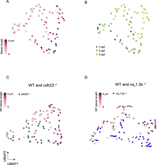
(A) UMAP plot of HCs based on principal component analysis of mitochondrial properties. Variables included in this analysis: (1) number of mitochondria, (2) total mitochondrial volume, (3) max mito volume, (4) max mito cable length, (5) median mito volume, (6) average minimum distance between max mito and ribbons, and (7) average minimum distance between median mito and ribbons. HCs are color-coded by stereocilia length. (B) Same UMAP analysis as in (A), color-coded according to age of the animal. Total HCs, n = 75. 3 days post fertilization (dpf) HC: n = 10, 2 NM, 2 fish. 5 dpf HCs: 38 HC, 3 NM, 2 fish. 6 dpf HC: n = 27 HC, 2 NM, 1 fish. (C) UMAP analysis comparing WT to cdh23 HCs. (D) UMAP plot comparing WT to cav1.3a HC. WT HC data, n = 75 HCs, 7 NM, 5 fish (3–6 dpf, same as A and B). cdh23 data, n = 19, 4 NM, 2 fish, 5 dpf. cav1.3a data, n = 45, 4 NM, 2 fish, 5 dpf.
|