(A) An adult wild type (WT) fish. Stripes and interstripes are labelled according to their order of temporal appearance. X0 is the first interstripe to appear. 1D and 1V (D - Dorsal, V- Ventral) are the first two stripes to appear. X1D and X1V are the next two interstripes to appear and so on. Image reproduced from Frohnhöfer et al., 2013 and licensed under CC-BY 4.0 (https://creativecommons.org/licenses/by/4.0). (B) Summary of pigment cell distribution in adult zebrafish. The cells in the xanthophore, S-iridophore, melanophore and L-iridophore layers consist of xanthophores and xanthoblasts, melanophores, S-iridophores and L-iridophores, respectively. Adapted from Hirata et al., 2003. (C) Schematic of WT patterns on the body of zebrafish. Stages PB, PR, SP, J+ correspond to developmental stages described in 3. Patterns form sequentially outward from the central interstripe, labelled X0, with additional dorsal stripes and interstripes labelled 1D, X1D, 2D, X2D from the centre (horizontal myoseptum) dorsally outward (similarly, ventral stripes and interstripes are labelled 1V, X1V, 2V, etc).

(A) An example model setup. The domain is made up of three layers. Layer 𝑿 which contains yellow X (yellow circles) and unpigmented Xb (clear circles with black outline). Layer 𝑰 which contains silvery Id (white circles) and blue Il (blue circles). Layer 𝑴 which contains black M (black circles) only. Each lattice site on each of the respective layers contain at most one cell at any given time. The layers are stacked on top of each other as seen in real fish. We note that in our simulations the ordering of the layers does not play any role in determining pattern formation. (B) Schematics of model implementation. (1) The model is initialised as described in Appendix 1. (2) The model is checked for the requirements for a fixed event to occur (e.g. new cells differentiating at a given time). If there is a fixed event to be implemented, the algorithm moves to stage 3. Otherwise, the algorithm passes to stage 4. (3) The model is updated according to the fixed event and algorithm returns to stage 2. (4) The propensity functions - probabilities for all other events to occur α1⁢(t),…⁢α15⁢(t) are calculated. (5) Random numbers u0,u1∈U⁢(0,1) are generated. (6) Numbers u0,u1 are used to determine the time τ until the next event and which event will be implemented. (7) The model configuration is updated. (8) The algorithm checks if the end criterion is satisfied, that is in the case of WT, that ΩSL=13.5mm. If so, the algorithm finishes. Otherwise the algorithm continues, returning to stage 2. (9) The simulation completes.

(A–F) Comparing the number of cells in the short (A–D) and long (E–F) range distance (0.04 mm) from a central site, on different domain types. M are represented as black circles. X are represented as yellow circles. (A–B) A visualisation of sites (marked in red) local to central melanocyte on the (A) melanocyte domain and (B) xanthophore domain.(C–D) A visualisation of sites (marked in red) local to central xanthophore on the (C) xanthophore domain and (D) melanocyte domain. (E–F) A visualisation of sites (marked in red) long-distance to central melanocyte on the (E) melanocyte domain and (F) xanthophore domain.(G–H) A visualisation of sites (marked in red) long-distance to central xanthophore on the (G) xanthophore domain and (H) melanocyte domain. (I) Melanophore movement with respect to local neighbours. If a melanophore located in a central position (marked in dark grey) attempts to move, the melanophore will consider neighbours in all sites marked in red on the melanophore domain (left), xanthophore and S-iridophore domain (right). (J) Movement on xanthophore/iridophore domain with respect to local neighbours. If a xanthophore/iridophore located in a central position (marked in dark grey) attempts to move, the xanthophore/iridophore will consider neighbours in all sites marked in red on the xanthophore and S-iridophore domain (left), melanophore domain (right).

(A–F) Adult phenotype of the set of fish used to deduce S-iridophore interactions. (A) WT fish, (B) shady (shd), (C) nacre(nac), (D) pfeffer (pfe), (E) nac;pfe, (F) shd;pfe. (G) A representation of all the interactions implemented in the model. See Supplementary files 4 and 5 for a detailed justification of the rates and interaction types, respectively. See Supplementary file 6 for a detailed justification of all parameters. The direction of the arrow/inhibition sign indicates which cell is acting on which. For example in assumption 13, the blue arrow from melanophore to xanthophore indicates that melanophores attract (green background) xanthophores. The purple inhibition arrow indicates that the xanthophores repel melanophores. OR statements in assumptions 15–18 are logical OR statements. For example, conditons 15 and 16 indicate that a dense S-iridophore may become loose if there are melanophores in the short range OR, there are no xanthophores in the short range AND many xanthophores in the long range. (H) A visualisation of measurements HAA and SL. (I) Plots of SL versus days post-fertilisation (dpf) for 40 model realisations. Each coloured line is a single realisation. Black squares are SL versus days post-fertilisation extracted from Parichy et al., 2009 in real fish given in Supplementary file 3. Red diamonds are the mean SL versus days post-fertilisation from 40 simulations. (J) Plots of SL (mm) versus HAA (mm) for 40 model realisations. Each coloured line is a single realisation. Black squares are SL versus HAA extracted from Parichy et al., 2009 given in Supplementary file 3. Red diamonds are the mean HAA versus SL from 40 simulations. Error bars are one standard deviation. The model agrees well with the data in both cases. Images (A–F) reproduced from Frohnhöfer et al., 2013 and licensed under CC-BY 4.0 (https://creativecommons.org/licenses/by/4.0).

(A–D), (E–H), (I–L), (M–P) WT, shd, nac, pfe development respectively and (A’–D’), (E’–H’), (I’–L’), (M’–P’) corresponding model simulation. Red arrows: melanocytes in the skin layer, modelled in (A). White arrows indicate the embryonic pattern of melanocytes in four stripes, that are deeper than the skin level and are consequently not included in the model. See Videos 1–4 for representative examples of these simulations in movie format. Scale bar is 0.25 mm for all images. Experimental images (A–D), (E–H), (I–L), (M–P) reproduced from Frohnhöfer et al., 2013 and licensed under CC-BY 4.0 (https://creativecommons.org/licenses/by/4.0).

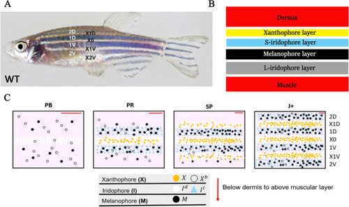
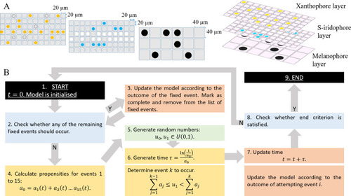
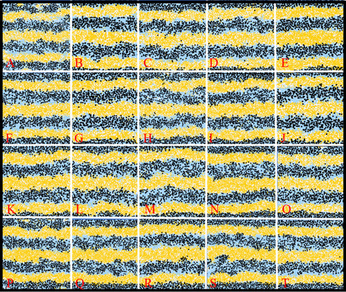
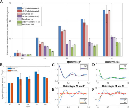
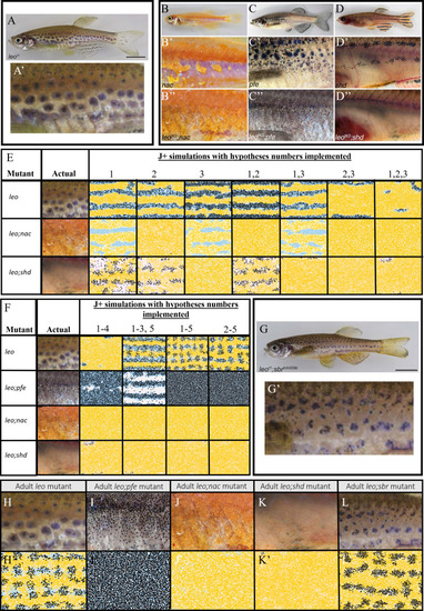
Each square is an example WT simulation at stage J+ where each rate parameter is perturbed to 1+x times its normal value. The value x is chosen uniformly at random from the set [-0.25,0.25].

(A–C) Real stage J+ shd;pfe, nac;pfe, shd;nac mutants, respectively. (A’–C’) Model simulations at stage J+ for shd;pfe, nac;pfe, shd;nac mutants, respectively. (D–F) Adult phenotype of selected (D) rse, (E) sbr, (F) cho mutant. (G–J), (K–N), (O–Q) rse, sbr and cho development, respectively. (G’–J’), (K’–N’), (O’–Q’) rse, sbr and cho model simulations, respectively. (R) seurat at stage J. (R’) seurat model simulation at stage J. Scale bar is 0.25 mm for all images. See Videos 5–7 for representative examples of these simulation in movie format. Experimental images (A–C), (D), (F) (G–J) and (O–Q) are reproduced from Frohnhöfer et al., 2013, (E), (K–N) from Fadeev et al., 2015, (R) from Eom et al., 2012 and are all licensed under CC-BY 4.0 (https://creativecommons.org/licenses/by/4.0).

(A–C) Regeneration of new pigment producing cells 7, 14 and 21 days respectively after a small rectangular window of cells in the adult WT stripes are completely ablated (Patterson and Parichy, 2013). (D–F) A representative simulation of the regeneration of an adult zebrafish 7, 14 and 21 days after a simulated ablation has occurred. Scale bar is 0.25 mm in all images. Experimental images (A–C) are reproduced from Yamaguchi et al., 2007. Copyright (2007) National Academy of Sciences U.S.A.; these images not covered by the CC-BY 4.0 licence and further reproduction of this panel would need permission from the copyright holder.

(A) S-iridophores are ablated using pnp4a:NTR+Mtz at stage PB (B) Stripe development in wild-type fish following S-iridophore ablation. Xanthophores are associated with S-iridophore interstripe. Melanophores aggregate around the new interstripe. (C–D) A representative simulation of S-iridophore ablation and subsequent development. For clarity, dense S-iridophores are displayed in green in (C). Scale bar is 0.25 mm in all images. Experimental images (A–B) are reproduced from Patterson and Parichy, 2013 and licensed under CC-BY 4.0 (http://creativecommons.org/licenses/by/4.0).

(A) Number of melanocytes per ventral hemisegment. Quantification of melanocytes. A comparison of melanocyte numbers between mutants and WT seen in our simulations and data recreated from Frohnhöfer et al., 2013. For each stage, our simulated number of melanocytes was normalised by the WT number in data by Frohnhöfer et al., 2013. (The number of animals used for counting was at least five for each measurement point.) The number of simulations was 100. Error bars indicate the standard deviation. There is no error bar for WT, since WT data was used to normalise the data. (B) X0 interstripe width. A comparison of X0 stripe width in 100 simulations with X0 stripe width in real mutants (taken from representative images; Frohnhöfer et al., 2013). The darker bars depict experimental data, lighter bars depict our simulated data. Error bars indicate the standard deviation. Since there is only one image for each of the respective mutants, there is no error bar for actual (real experimental data). (C–F) PCF for different cell types averaged over 100 simulations using the square uniform PCF (Gavagnin et al., 2018). The spatial pair correlation as a function of distance for (C) dense S-iridophores only (D) melanocytes only, (E) melanocytes and dense S-iridophores, (F) melanocytes and xanthophores. Experimental data in (A) is reproduced from Frohnhöfer et al., 2013.

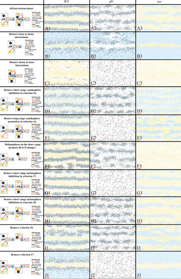
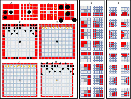
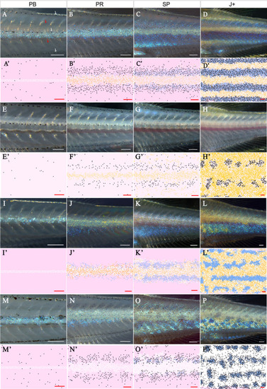
The first column displays a diagram of the S-iridophore interactions which remain (all other cell-cell interactions are unchanged). Columns 2–4 are representative simulations of WT, pfe and nac under these conditions. *This interaction is equivalent to removal of long range xanthophore inhibition in criterion 17. It is also equivalent to removal of short range xanthophore promotion in criterion 18.

(A–B) WT and shd respectively with all rules included. (C–D) No movement of melanocytes or xanthophores for WT and shd, respectively. (E) Differentiation of melanocytes only promoted by dense S-iridophores for WT fish that is the rate of melanocytes does not depend on the number of S-iridophores. (F–G) No pull of melanocytes by xanthoblasts for WT and shd fish, respectively. (H) No proliferation of xanthophores for WT. (I–J) No melanocyte death for WT and shd fish. (K) Differentiation of melanocytes is not dependent on S-iridophores, (L–M) No death of melanocytes for WT and shd (N) Differentiation of melanocytes is dependent on dense S-iridophores being present in the long distance only.

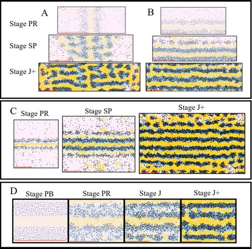
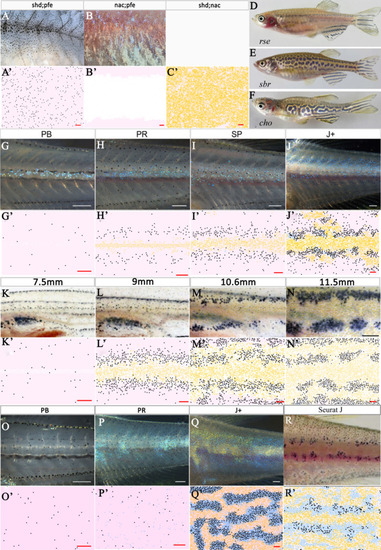
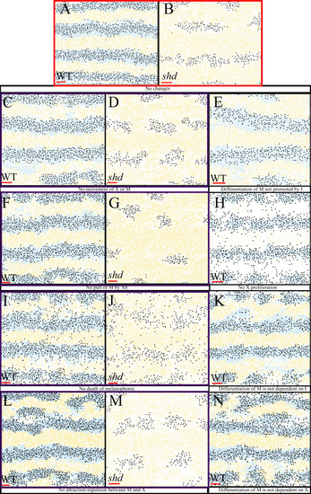
The simulated domains at stages PR, SP and J+ wherein the following are changed (A) the orientation of the initial S-iridophore interstripe, (B) the initial position of the S-iridophore interstripe, (C) the initial domain size (D) the initial domain so that it is populated with adult-width stripes and interstripes.

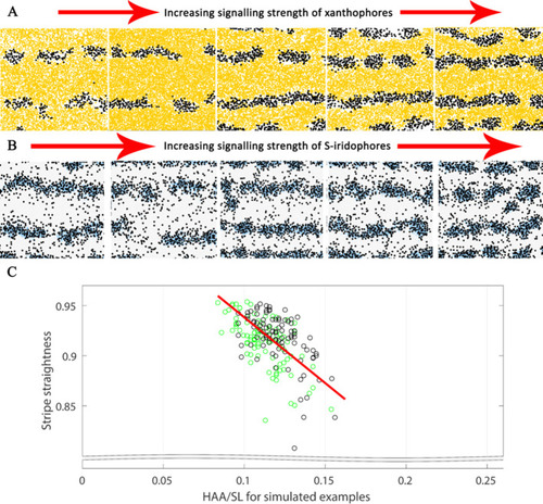
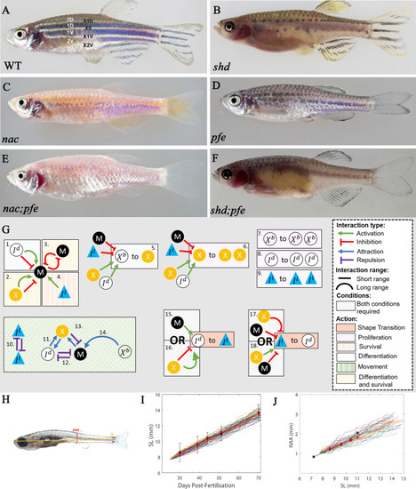
The effects of different signalling strengths in pfe and shd. Representative images of J+ simulations of (A) shd and (B) pfe where the signalling strength of melanocyte differentiation in the long range is increased (from left to right). Increasing the signalling strength of the respective cell types decreases the width of the interstripe X0 and increases the number of pseudo-stripes from 2 to 4. For our simulations, we choose the weakest shown signalling strength for xanthophores, corresponding to the furthest left of (A) and the strongest shown signalling strength for S-iridophores, corresponding to the furthest right of (B). (C) Stripe straightness of our simulations correlates with the simulated HAA/SL ratio. Each circle is one simulation, green circles indicate simulations up to stage J, black circles indicate simulations of up to stage J+. There are one hundred simulations in total for each stage. The red line is the line of best fit.

(A–D) Adult leo, nac, pfe and shd respectively. (A’–D’) The flanks of leo, nac, pfe and shd respectively. (B’’–D’’) The flanks of leo;nac, leo;pfe and leo;shd respectively. (E) Example simulations where combinations of hypotheses 1–3 in the text are implemented. (F) Example simulations where combinations of hypotheses 1–5 in the text are implemented. Note that simulations of 1–5 are similar to simulations for 2–5, indicating that hypotheses one is not necessary to predict the leo phenotype. (G) Adult leo;sbr (G’) Flank of leo;sbr. (H–L) Adult mutants contrasting with (H’–L’) simulations using hypotheses 1–5 from the main text. (H–L) Flank of leo, leo;nac, leo;pfe, leo;shd and leo;sbr respectively. (H’–L’) Simulated images of leo, leo;pfe, leo;nac, leo;shd and leo;sbr respectively at stage J+. (A), (A’), (G), (G’), (H) and (L) from Fadeev et al., 2015, (B–D’’), (I–K) from Irion et al., 2014 and are all licensed under CC-BY 4.0 (http://creativecommons.org/licenses/by/4.0).