Overview of segmentation and shape parameterization. (A) Representative maximum intensity projections (left column) and corresponding 3D projections (right column) for nuclei labeled with DRAQ5 dye (top row), cells labeled by Tg(-8.0cldnb:LY-EGFP) (middle row) and both channels together (bottom row). (B) Image depicting how the first rotation angle is calculated. Example given for the maximum intensity projection segmentation channel of the neuromast shown in A. Cells 1, 2 and 3 are used in C and D. (C) Example of the alignment procedure as applied to cell 1 from B. To correct for radial symmetry, cells are first rotated around the z-axis. Cells were then rotated around the y-axis to correct for apicobasal tilt, and then around the x-axis to correct for off-parallel tilt during imaging. (D) Overview of shape parameterization using SH, as applied to cells 1, 2, and 3 from B. SH expansion is applied to original 3D surface meshes (left) to generate the cell-by-SHE coefficients table (middle), which can then be used to generate 3D reconstructions (right).

Visualization of cell shape modes 1 and 2. (A) Schematic depicting how shape variation was visualized. PCs were first z-scored to generate shape modes. Visual representations of each shape mode were generated by finding the mean cell (a hypothetical cell with a value of 0 for all 8 shape modes) and varying one shape mode (here, shape mode 1) by up to 2 standard deviations (s.d.) while holding other shape modes at the mean (0). (B) Schematic depicting how relative cell locations within each neuromast were calculated. The distance between the neuromast centroid and the furthest cell (r) in the xy plane was calculated. The distances between the neuromast centroid and cell centroids were divided by (r) to yield the normalized distance from the neuromast center (d). The angular location of each cell was determined in reference to the positive x-axis centered on the neuromast centroid. Cell locations were projected onto a unit circle with radius 1. (C) Visualization of CSM1, generated as described in A. 3D surface renderings are shown from three different views, as well as an overlay of point representations for each view (rightmost column). (D) Polar plots of relative cell locations (generated as shown in B) binned by CSM1 scores. Bins were centered on the corresponding z-score and included cells with values within 0.5. For the −2 s.d. and 2 s.d. plots, the upper bounds were not limited to within 0.5 (e.g. the first plot includes all cells with CSM1 values less than −1.5 s.d.). An overlay of the first five plots is shown in the rightmost column. (E) Visualization of CSM2. 3D surface renderings are shown from three different views, as well as an overlay of point representations for each view (rightmost column). (F) Polar plots of relative cell locations binned by CSM2 scores. An overlay of the first five plots is shown in the rightmost column.

Visualization of nuclear shape modes 1 and 2. (A) Visualization of NSM1, generated as in Fig. 2A. 3D surface renderings are shown from three different views, as well as an overlay of point representations for each view (rightmost column). (B) Polar plots of relative cell locations (generated as in Fig. 2D) binned by NSM1 scores. An overlay of the first five plots is shown in the rightmost column. (C) Visualization of NSM2. 3D surface renderings are shown from three different views, as well as an overlay of point representations for each view (rightmost column). (D) Polar plots of relative cell locations binned by NSM2 scores. An overlay of the first five plots is shown in the rightmost column.

Unsupervised clustering of cells in shape space. (A) UMAP of neuromast cells, color coded by cell shape cluster. Colors and associated cluster numbers are used in B-F. (B) PAGA plot of cell shape clusters. Each node represents a cluster. Thickness of the line drawn between nodes indicates estimated connectivity between clusters (the value of which is shown adjacent to the corresponding line). Edges with connectivity below 0.1 are not depicted. (C) 3D projections of representative cells for each cluster, defined as the cell closest to the cluster centroid in eight-dimensional PC space. (D) Polar plots of relative neuromast locations of cells within each cluster. (E) Distributions of the cell distance from the neuromast center for each cluster. Dashed lines indicate quartiles. (F) Distributions of neuromast cell angles for each cluster. Dashed lines indicate quartiles. Angles were calculated with reference to the positive x-axis extending from the neuromast centroid. Cluster 1 shows a bias towards the dorsoventral poles (90° and −90°), whereas cluster 2 shows a bias to the anterior-posterior compartments (0°, 180° and −180°).

Unsupervised clustering of nuclei in shape space. (A) UMAP of neuromast cells, color coded by nucleus shape cluster. Colors and associated cluster numbers are used in B-F. (B) PAGA plot of nucleus shape clusters. Each node represents a cluster. The thickness of the line drawn between nodes indicates the estimated connectivity between clusters (the value of which is shown adjacent to the corresponding line). Edges with connectivity below 0.1 are not depicted. (C) 3D projections of representative cells for each nuclear cluster, defined as the cell closest to the cluster centroid in four-dimensional PC space. The original segmentation masks are depicted (not SHE reconstructions). (D) Polar plots of relative locations of cells within each cluster. (E) Distributions of the cell distance from the neuromast center for each cluster. Dashed lines indicate quartiles. (F) Distributions of neuromast cell angles for each cluster. Dashed lines indicate quartiles. Angles were calculated with reference to the positive x-axis extending from the neuromast centroid.

Location and shape characteristics of cells expressing sost:NLS-Eos and sfrp1a:NLS-Eos. (A) Single confocal slice of a neuromast from sost:NLS-Eos; Tg(-8.0cldnb:LY-EGFP) fish stained with DRAQ5. Image contrast was adjusted for visibility. (B) The same slice as in A, with the sost:NLS-Eos channel (gray) overlaid with a mask indicating cells classified as Eos⁺ (cyan). (C) Polar plot showing relative cell locations of locations of Eos⁺ (cyan) and Eos⁻ (gray) cells. (D) UMAP of Eos⁺ (cyan) and Eos⁻ (gray) cells from sost:NLS-Eos. (E) sost:NLS-Eos⁺ cells plotted as raw counts within each cell shape cluster. (F) sost:NLS-Eos⁺ cells plotted as the percentage of each cluster. (G) Single confocal slice of a neuromast from sfrp1a:NLS-Eos; Tg(-8.0cldnb:LY-EGFP) fish stained with DRAQ5. Image contrast was adjusted for visibility. (H) The same slice as in A, with the sfrp1a:NLS-Eos channel (gray) overlaid with a mask indicating cells classified as Eos⁺ (cyan). (I) Polar plot showing relative cell locations of locations of Eos⁺ (cyan) and Eos⁻ (gray) cells. (J) UMAP of Eos⁺ (cyan) and Eos⁻ (gray) cells from sfrp1a:NLS-Eos. (K) sfrp1a:NLS-Eos⁺ cells plotted as raw counts within each cell shape cluster. (L) sfrp1a:NLS-Eos⁺ cells plotted as the percentage of each cluster.

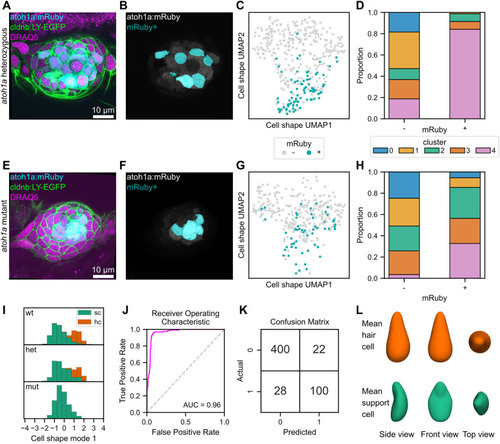
Shape characteristics of atoh1a:mRuby heterozygotes and mutants, and logistic classifier for hair cells based on cell shape features. (A-G) Analysis of cell shape distributions in atoh1a:mRuby heterozygotes (A-D) and mutants (E-H). (A,E) Single confocal slice of a neuromast from an atoh1a:mRuby heterozygote (A) and mutant (E) also expressing Tg(-8.0cldnb:LY-EGFP) and stained with DRAQ5. Image contrast was adjusted for visibility. (B,F) The same slices as in A and E, with the atoh1a:mRuby channel (gray) overlaid with a mask indicating cells classified as mRuby⁺ (cyan) for a atoh1a:mRuby heterozygote (B) and mutant (F). (C,G) UMAP of mRuby⁺ (cyan) and mRuby⁻ (gray) cells from atoh1a:mRuby heterozygotes (C) and mutants (F). (D,H) Proportions of mRuby⁻ cells (left bar) and mRuby⁺ cells (right bar) from atoh1a:mRuby heterozygotes (D) and mutants (H) in each cell shape cluster. (I) Distributions of cell shape mode 1 scores, separated by genotype (top row, wild type; middle row, atoh1a heterozygous; bottom row, atoh1a mutant). Hair cells (hc, green); support cells (sc, orange). (J) Receiver operating characteristic (ROC) curve (fuchsia) for a logistic regression classifier trained to detect hair cells based on cell shape mode 1-8. The area under the curve (AUC) score is shown (0.96). Gray dashed line, performance of a random classifier. (K) Confusion matrix for the cell shape-based hair cell classifier. 0, support cells; 1, hair cells. Top left, true negatives; top right, false positives; bottom left, false negatives; bottom right, true positives. (L) The idealized mean cell shape for hair cells (top, orange) and support cells (bottom, green).