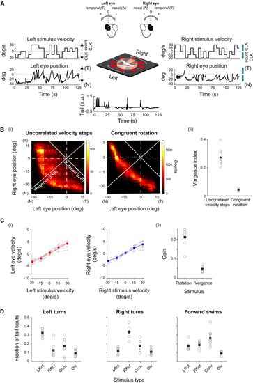
Split motion stimuli are used to decouple eye movements

(A) Schematic of visual stimulation (center). Eye rotations are elicited by rotating radial patterns, split into two hemifields, and projected onto a screen placed below the fish (see Video S1). Both eye and tail positions are tracked during stimulus viewing.

(B) (i) Left and right eye positions are decorrelated when using a split stimulus (left, uncorrelated velocity steps). In comparison, they are highly correlated when using a whole-field rotating grating (right, congruent rotation). (ii) Vergence index for fish presented with split, incongruent motion stimuli (8 fish) and congruent rotation stimuli (5 fish). Filled circles, mean across fish. Open circles, individual fish.

(C) Eye velocity is modulated by stimulus velocity (see also Figure S1). (i) Left eye and right eye velocities (saccades removed) for each stimulus velocity presented on the ipsilateral side of the screen. Red and blue points, mean across fish (N = 8); gray traces, individual fish. The slope of the fitted lines reflects the eye velocity gain, i.e., the modulation of eye velocity by stimulus velocity. (ii) Eye velocity gain, pooled for both eyes, for stimuli grouped into rotating and vergent. Filled circles, mean across fish (n = 8). Open circles, individual fish (see STAR Methods and Figure S1D).

(D) Swimming bout type is modulated by stimulus category (see also Figure S1A). Filled circles, mean across fish (n = 8). Open circles, individual fish. Conv, converging; Div, diverging; LRot, leftward rotation (counterclockwise); RRot, rightward rotation (clockwise).

See also Figure S1 and Video S1.

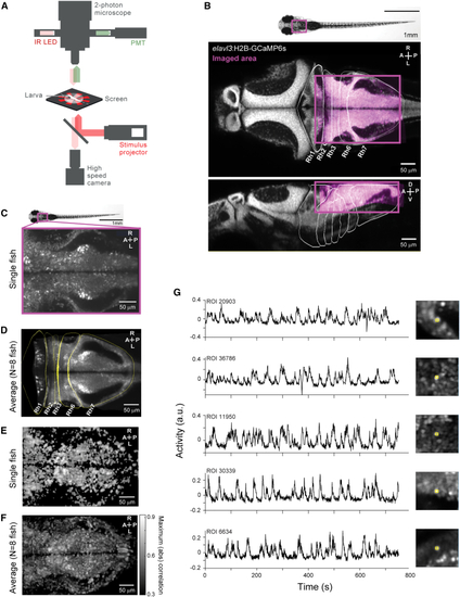
Activity related to behavior is widespread in the zebrafish hindbrain

(A) Schematic of experimental setup (see STAR Methods), showing simultaneous brain imaging, behavior monitoring, and visual stimulus presentation.

(B) Representative plane highlighting the imaged region (magenta) overlaid on the corresponding plane of the Z-brain atlas.⁴⁷ Top, dorsal view. Bottom, sagittal view.

(C) Example plane of the imaged area in a representative fish.

(D) Example plane of the average image stack across eight fish (see STAR Methods).

(E) Maximum absolute correlation value with any of the expanded set of behavioral regressors (see STAR Methods) for an example fish (maximum projection of the imaged stack).

(F) Average maximum absolute correlation maps across eight fish, after registration to an internal template (see STAR Methods; maximum projection of average stack). Correlation maps are thresholded at 0.3 absolute correlation value.

(G) Example traces of ROIs used in the analysis.

See also Table S1, and Video S2.

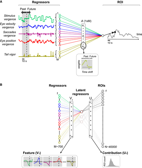
Regression models

(A) Multiple linear regression model for a single ROI. For each original variable (only a subset shown here, see Figure S2), the regression model finds a set of weights that corresponds to the contribution of the variable at different time points (gray window, left) to ROI activity at the present time point (black dot, right). Inset shows the weights for one of the variables. Dotted line corresponds to no time-shift.

(B) Reduced-rank regression. Each time-shifted regressor is first mapped onto a set of latent regressors. The pattern of weights (V₁) that determines the mapping for one latent regressor is called a feature (left inset, each regressor is represented in one color). In turn, the latent regressor is associated with a pattern of ROI activity, determined by its contribution weights (U₁). Right inset shows distribution of the U₁ values (U₁ contribution) for this example feature. This distribution illustrates how strongly the latent regressor associated with this feature is expressed across the population.

See also Figures S2 and S3.

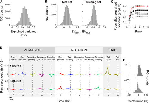
Activity is explained by a small number of features that separate vergence and rotation variables

(A) Explained variance (EV; cross-validated) for the ROIs of an example fish using RRR.

(B) The cross-validated explained variance of the best RRR model (EV_RRR) was generally higher than the explained variance of the best MLR model (EV_MLR) (left). Right shows performance on training data, i.e., without cross-validation. Same fish as in (A).

(C) Population-explained variance (popEV, cross-validated; see STAR Methods) as a function of the number of features (rank) included in the model for each individual fish (gray traces; example fish in A and B is shown in red) and across fish (average of 8 fish, black trace; error bars correspond to SEM).

(D) The first two features for the example fish. Feature traces are scaled by their overall importance (V^∗S; see STAR Methods). For each feature, variables are color-coded and sorted into vergence, rotation, and tail variables. Vertical dotted line indicates a time shift of zero. Traces of five cross-validation runs are shown and closely overlap. Note that feature 1 groups activity related to vergence and swimming, whereas feature 2 groups activity related to rotation. Features 3–6 of this fish have only a minor contribution to the popEV (see Figure S5).

(E) Contribution of the latent regressors associated with features 1 (vergence) and 2 (rotation) to ROI activity for the same example fish (43,622 ROIs).

See also Figures S4 and S5.

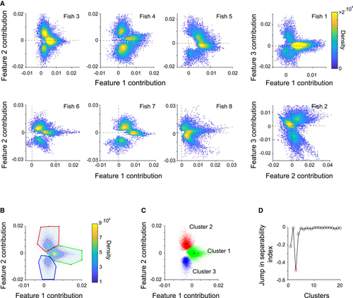
Equivalent ROI clusters are found across all imaged fish

(A) Contributions (U) to ROI activity of latent regressors associated with vergence and rotation features group into three clusters. Each dot corresponds to an ROI, each panel to a different fish. Only ROIs with EV > 0.4 are included.

(B) Manual assignment of ROIs to three clusters in feature contribution (U₁-U₂; see STAR Methods) space for an example fish (STAR Methodsbased on the density plot.

(C) ROIs for the example fish are color-coded according to their cluster assignment (ROIs are subsampled here for better visualization). Black asterisks mark cluster centroids.

(D) Using ClusterDv⁵¹ (see STAR Methods) we also find three clusters.

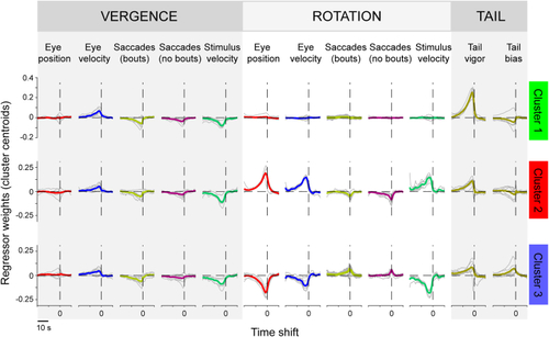
Clusters relate to vergence and left/right rotational motion

The weighted contribution of features 1–3 is shown for each cluster’s centroid. Each row corresponds to a cluster, and variables are grouped into vergence, rotation, and tail variables (compare to Figure 4D). Cluster 1 (green) is composed exclusively of vergence variables and swimming. Clusters 2 (red) and 3 (blue) relate to leftward and rightward rotation, respectively. Gray traces, individual fish. Color traces, mean across seven fish (one fish was excluded here because the tail tracking was too noisy).

See also Figure S6.

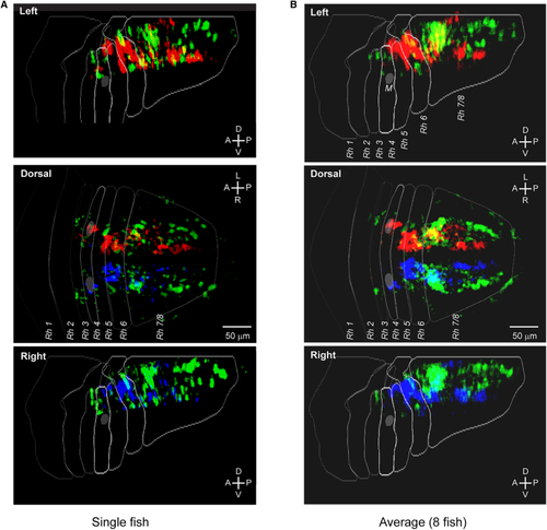
Anatomical distribution of ROIs belonging to the vergence and rotation clusters

(A) Spatial distribution of the ROIs assigned to the three clusters in the example fish (32,228 ROIs with EV > 0.4).

(B) Average distribution of the ROIs assigned to the three clusters (n = 8 fish). Individual maps (see Figure S7) were registered to the Z-brain template before averaging. Scale bar, 50 μm. Dark gray ellipse shows the location of the Mauthner cells (M). Rhombomere contours and Mauthner cell correspond to Z-brain masks.⁴⁷

See also Figure S7 and Video S3.