
- Title
-
Neuronal birthdate reveals topography in a vestibular brainstem circuit for gaze stabilization
- Authors
- Goldblatt, D., Huang, S., Greaney, M.R., Hamling, K.R., Voleti, V., Perez-Campos, C., Patel, K.B., Li, W., Hillman, E.M.C., Bagnall, M.W., Schoppik, D.
- Source
- Full text @ Curr. Biol.
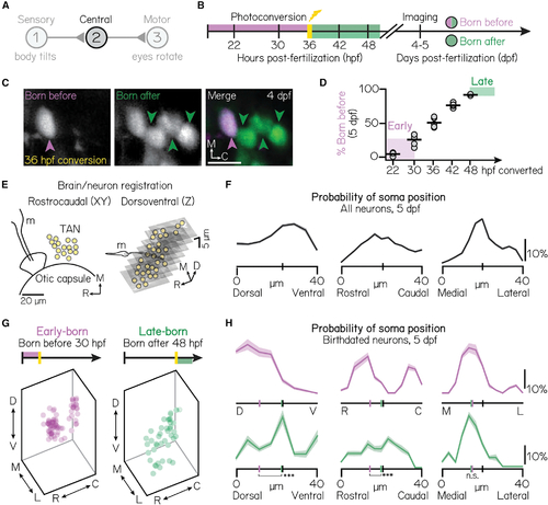
Projection neuron birthdate predicts soma position
(A) Schematic of the vestibulo-ocular reflex circuit used for gaze stabilization. (B) Timeline of birthdating experiments. Neurons born by the time of photoconversion have both magenta (converted) and green (unconverted) Kaede. Neurons born after photoconversion have exclusively green (unconverted) Kaede. All fish are imaged well after photoconversion, at 4–5 days post-fertilization (dpf). (C) Example projection neurons photoconverted at 36 hpf, visualized using the Tg(−6.7Tru.Hcrtr2:GAL4-VP16; UAS-E1b:Kaede) line. Magenta and green arrows indicate neurons born before or after 36 hpf, respectively. Scale bars (white), 20 μm.). (D) Percent of projection neurons born at each time point. Black lines indicate the mean percent across individual fish (circles). Shaded bars indicate cohorts designated as early-born (converted by/born before 30 hpf) or late-born (unconverted at/born after 48 hpf). n = 5 hemispheres/time point from at least N = 3 larvae (22–42 hpf) or n = 3 hemispheres from N = 3 larvae (48 hpf).). (E) Schematic of brain/neuron registration in the rostrocaudal/xy (left) and dorsoventral/z (right) axes. Black solid lines outline anatomical landmarks used for registration. Yellow circles indicate the position of individual projection neurons. m, Mauthner neuron.). (F) Soma positions of n = 660 registered neurons from N = 10 non-birthdated fish at 5 dpf. Probability distributions shown are the mean (solid) and standard deviation (shaded outline) after jackknife resampling. Short vertical axis lines indicate the median position of all registered neurons.). (G) Soma position of birthdated projection neurons. Early-born (left): n = 74 neurons from N = 7 fish. Late-born (right): n = 41 neurons from N = 10 fish.). (H) Same data as Figure 1G, shown as probability distributions for each spatial axis. Distributions shown are the mean (solid) and standard deviation (shaded outline) after jackknife resampling. Short vertical axis lines indicate the median position of early- (magenta) or late-born (green) projection neurons, compared with control distributions shown in Figure 1F (black). ***difference between the early- and late-born probability distributions at the p < 0.001 level; *significance at p < 0.05; n.s., not significant.). See also Figure S1. |
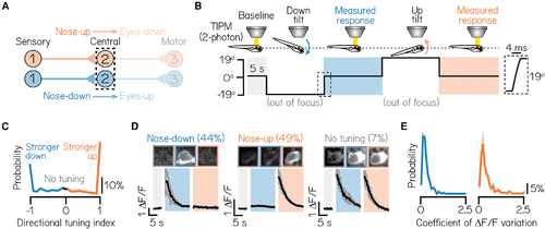
Pitch-tilt rotations reliably differentiate two cardinal subtypes of projection neurons
(A) Circuit schematic for pitch-tilt rotation experiments. Black dashed lines outline projection neurons as circuit population of focus. (B) Schematic of pitch-tilt rotation stimulus and imaging using Tilt In Place Microscopy (TIPM) and a two-photon microscope. Shaded regions show time of measured responses following nose-down or nose-down tilts. Inset shows a feedback trace from the galvonometer during the restoration step to horizontal. (C) Distribution of the directional tuning for all sampled neurons. Gray region indicates neurons with no directional tuning; blue and orange regions indicate neurons with stronger nose-down or nose-up responses, respectively. Criteria are detailed in STAR Methods. Solid line shows mean from jackknife resampling; shaded bars, standard deviation. (D) Example images and traces of a nose-down projection neuron (left), nose-up projection neuron (middle), and a projection neuron with no directional tuning (right) during TIPM. Projection neurons are visualized using the Tg(−6.7Tru.Hcrtr2:GAL4-VP16) line and express a UAS:GCaMP6s calcium indicator. Solid black lines show mean response across three stimulus repeats and shaded lines, standard deviation. Parentheses indicate the percent of neurons with each subtype, n = 467 neurons, N = 22 fish. (E) Distributions of the coefficient of variation of peak Δ F/F responses across three stimulus repeats for nose-down (left) and nose-up (right) neurons. Solid lines show mean from jackknife resampling; shaded bars, standard deviation. See also Figures S2 and S3. |
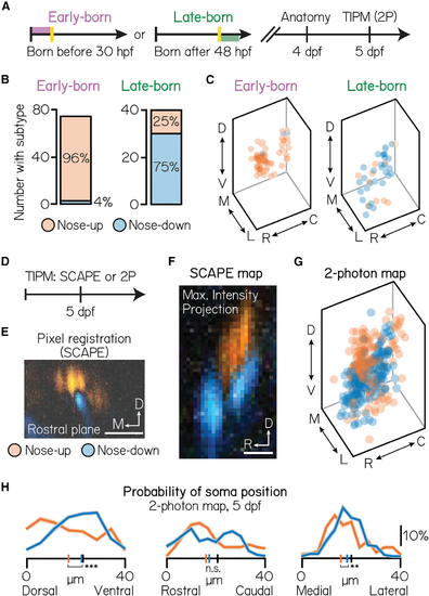
Birthdating reveals functional somatic topography to projection neurons
(A) Timeline of functional birthdating experiments. Larvae were birthdated at either 30 or 48 hpf and then imaged on a confocal (4 dpf) and two-photon (5 dpf) to identify projection neuron soma position, birthdate, and directional (up/down) identity. Projection neurons were visualized using the Tg(−6.7Tru.Hcrtr2:GAL4-VP16) line and expressed both the UAS:Kaede and UAS:GCaMP6s indicators. (B) Number of early- (left) and late-born (right) projection neurons with each directional subtype identity. Data from same neurons shown in Figure 1. (C) Soma position of early- (left) and late-born (right) neurons, pseudocolored according to directional identity. Data from same neurons shown in Figure 1. (D) Timeline of topography validation experiments. TIPM was performed on non-birthdated larvae at 5 dpf as shown in Figure 2B, using either a SCAPE or two-photon microscope. Projection neurons were visualized using the Tg(−6.7Tru.Hcrtr2:GAL4-VP16) line and expressed only the UAS:GCaMP6s indicator. (E) Registration method for SCAPE experiments. Pixels are pseudocolored according to the direction that evoked a stronger response. One example rostral plane shown. (F) Maximum intensity projection of the entire tangential nucleus from one fish imaged with SCAPE, pseudocolored as described in Figure 3E. (G) Soma position of neurons imaged with two-photon TIPM, pseudocolored by directional identity. Soma registered using method shown in Figure 1E. Data from the same n = 467, N = 22 fish as in Figures 2C–2E. (H) Probability of soma position for nose-up (orange) and nose-down (blue) projection neurons from two-photon TIPM. Distributions shown are the mean (solid) and standard deviation (shaded outline) after jackknife resampling. Short vertical axis lines indicate the median position of up/down projection neurons, compared with control distributions shown in Figure 1F (black). ***difference between the nose-up and nose-down distributions at the p < 0.001 level; **significance at p < 0.01; n.s., not significant. See also Figure S4. |
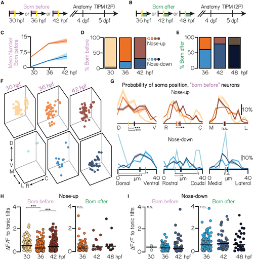
Projection neurons are assembled into the tangential nucleus in a stereotyped temporal sequence
(A) Timeline of functional birthdating experiments. Only projection neurons born before the time of conversion (red, converted Kaede) were analyzed. Projection neurons were visualized using the Tg(−6.7Tru.Hcrtr2:GAL4-VP16) line and expressed both the UAS:Kaede and UAS:GCaMP6s indicators. (B) Timeline of experiments. Only projection neurons born after the time of conversion (green, unconverted Kaede only) were analyzed. (C) Mean number of nose-up and nose-down neurons born before each age. Distributions shown are the mean (solid) and standard deviation (shaded outline) after jackknife resampling. (D) Percent of nose-up and nose-down neurons born before each age. Orange shades, nose-up; blue shades, nose-down. 30 hpf data are from the same N = 7 fish as in Figures 1G, ,1H,1H, ,3B,3B, and and3C.3C. 36 hpf: n = 208 sampled “born before” neurons from N = 7 fish; 42 hpf: n = 198 sampled born before neurons from N = 5 fish. (E) Percent of sampled nose-up and nose-down neurons born after each photoconversion time point. Orange shades, nose-up; blue shades, nose-down. 36 hpf: n = 168 born after neurons from N = 7 fish; 42 hpf: n = 66 born after neurons from n = 5 fish. 48 hpf data same as in Figures 1G, ,1H,1H, ,3B,3B, and and33. (F) Soma position of neurons born before each age. 30 hpf: all data shown. 36 hpf: n = 150/208 randomly selected neurons shown. 42 hpf: n = 150/198 randomly selected neurons shown. (G) Probability of soma position for all born before neurons. Distributions shown are the mean (solid) and standard deviation (shaded outline) after jackknife resampling. Short vertical axis lines indicate the median position of all birthdated neurons, compared with control distributions shown in Figure 1F (black). (H) Maximum change in calcium fluorescence to tonic tilts for nose-up neurons born before (left) or after (right) each age. Each circle represents a unique neuron. Solid line shows the mean across neurons. (I) Maximum change in calcium fluorescence to tonic tilts for nose-down neurons born before or after each age. All data: ***difference at the p < 0.001 level; **significance at p < 0.01; §, significance between p = 0.08 and p = 0.05; n.s., not significant. |
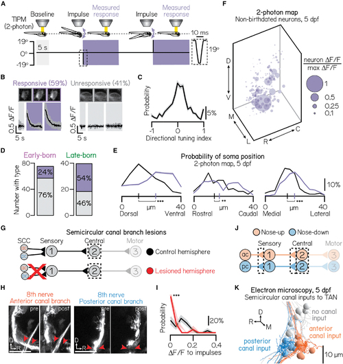
Birthdate reveals topography to semicircular canal-mediated, high-frequency stimulation responses (A) Impulse stimulus waveform. Shaded bars indicate time in the horizontal calcium imaging plane. Dotted box shows zoom of 10 ms impulse. (B) Example traces from an impulse-responsive (left) and unresponsive (right) projection neuron. Parentheses show percent of neurons in sample. Same n = 467 neurons, N = 22 fish as (C) Probability of directional selectivity to impulses. Zero indicates no directional preference. Distribution shows mean (solid line) and standard deviation (shaded outline) from jackknife resampling. (D) Number of early- and late-born projection neurons with (purple) or without (gray) impulse responses (purple). Data from same fish as in (E) Probability of soma position for impulse-responsive (purple) or unresponsive (gray) neurons from non-birthdated, two-photon TIPM; same n = 467 neurons, N = 22 fish as (F) Soma position of impulse-responsive neurons, scaled by impulse response strength (Δ F/F) relative to the strongest response observed. Larger circles indicate stronger responses. Data from the same neurons shown in (G) Circuit schematic. Both the anterior and posterior semicircular canal branches of the VIIIth nerve are uni-laterally lesioned. Calcium responses of projection neurons (black dashed box) in lesioned and control hemispheres are compared. (H) Example images from larvae before and after unilateral VIIIth nerve lesions. Left and right image sets (replicated from (I) Probability distributions of the maximum Δ F/F response to impulse rotations in lesioned (red) and control (black) hemispheres. Responses shown only for the most ventral 15 μm of projection neurons. Solid lines show mean from jackknife resampling; shaded bars, standard deviation. Control: n = 68 impulse responses, N = 3 fish. Lesioned: n = 132 impulse responses, N = 3 fish. (J) Circuit schematic for electron microscopy experiments. Black dashed lines indicate the circuit elements of focus: synaptic connections from the anterior and posterior semicircular canals to first-order sensory neurons, synaptic connections from sensory neurons to projection neurons, and projection neurons. (K) Electron microscopy reconstruction of 19 projection neurons at 5 dpf. Soma pseudocolored based on innervation from sensory neurons that receive anterior semicircular canal input (orange) or posterior semicircular canal input (blue). Gray soma receive no semicircular canal input. All panels: ***difference at the p < 0.001 level; **significance at p < 0.01. See also |
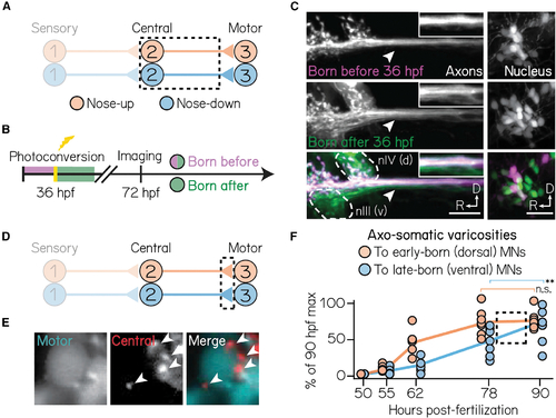
Birthdate predicts patterns of axonal trajectories and synapse formation between projection neurons and extraocular motor neurons
(A) Circuit schematic for axon birthdating experiments. Black dashed lines outline projection neuron soma and axonal projections to the extraocular motor nuclei. (B) Timeline of axon birthdating experiments. Larvae are only photoconverted at 36 hpf. (C) Birthdated axons from one example fish. Top row shows axons (left) from soma (right) born by 36 hpf; middle row shows axons that were not born by 36 hpf; bottom row shows merge. White arrows point to the ventral axon bundle. Inset shows zoom of axons. Dotted lines outline extraocular motor neuron somata. Scale bars, 20 μm. (D) Circuit schematic for synapse formation measurements. Black dashed lines outline axo-somatic varicosities from projection neurons onto post-synaptic ocular motor neurons. (E) Example image of an extraocular motor neuron (left) and axo-somatic varicosities (middle); right image shows merge. White arrows point to four example varicosities. Scale bars, 5 μm. (F) Rate of varicosity growth to early- and late-born ocular motor neurons, quantified as as a percentage of the maximum number of varicosities observed at 90 hpf. Circles represent individual fish. Dotted box highlights the time where the rate of varicosity formation to motor neuron subtypes diverges. n ≥ 5 fish per time point. **difference at the p < 0.01 level; n.s., not significant. |
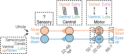
A model for the spatiotemporal organization of the gaze stabilization circuit
Spatiotemporal development of neurons that mediate the nose-up/eyes-down (orange) and nose-down/eyes-up (blue) gaze stabilization reflexes. nIII refers to the oculomotor cranial nucleus; nIV to the trochlear cranial nucleus IV. |