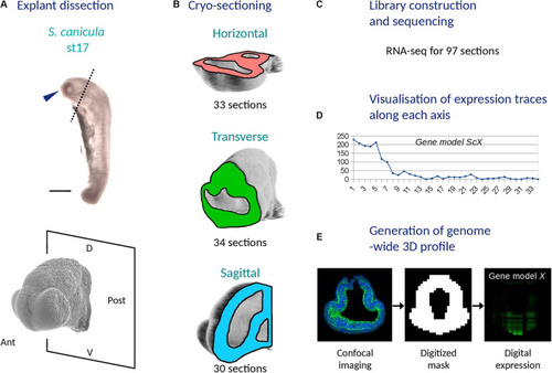
Main experimental steps used to generate a 3D RNA profile of the catshark embryonic head (stage 17). (A) Explant dissection: the top panel shows a left side photograph of a stage 17 catshark embryo with a blue arrowhead showing the dissected explant and a dotted line delimiting its posterior boundary and the bottom panel shows a higher magnification confocal view of the explant with the posterior dissection plane. (B) Cryo-sectioning: schemes show the planes used to generate series of cryo-sections (horizontal, pink; transverse, green; sagittal, blue). The total number of sections along each plane is indicated. (C) Library construction and sequencing resulting in RNA-seq data for a total of 97 sections. (D) Visualization of expression traces along each axis for all gene models. (E) Generation of a genome-wide 3D profile with its three steps (acquisition of a confocal 3D image of the explant, generation of a digitized model and computation of digital expressions for each voxel and gene model). D, dorsal; V, ventral; Ant, anterior; Post, posterior.

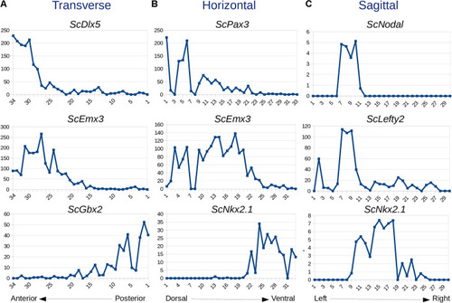
Expression traces for selected genes along transverse (A), horizontal (B), and sagittal (C) planes. For each graph, section numbers and corresponding read counts are indicated along x- and y-axes, respectively. Sections 1–34, 1–33, and 1–30 are, respectively, numbered from posterior to anterior in (A), dorsal to ventral in (B), and left to right in (C). Gene names are indicated at the top of each profile.

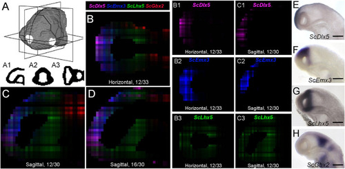
Digital profiles reproduce regional patterns along AP axis. (A) Scheme representing the digitized model of stage 17 catshark head with sagittal, transverse and horizontal digital section planes shown as white rectangles. (A1,A2,A3) show examples of digitized sections along these planes. (B–D) Digital horizontal (B) and sagittal (C,D) sections showing merged profiles of ScDlx5 (magenta), ScEmx3 (blue), ScLhx5 (green), and ScGbx2 (red). Sections are numbered from dorsal to ventral in panel (B) and from left to right in panels (C,D). (B1–3,C1–3) Digital sections showing the individual profiles, respectively, merged in panels (B,C) for ScDlx5(B1,C1), ScEmx3(B2,C2), and ScLhx5(B3,C3). (E–H) Left lateral views of stage 17 catshark embryonic heads after ISH with probes for ScDlx5(E), ScEmx3(F), ScLhx5(G), and ScGbx2(H). Scale bars = 200 μm.

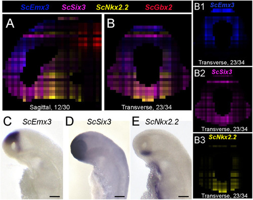
Digital profiles reproduce regional patterns along DV axis. (A,B) Digital sagittal (A) and transverse (B) sections showing merged profiles of ScEmx3 (blue), ScSix3 (magenta), ScNkx2.2 (yellow), and ScGbx2 (red). Sections are numbered from left to right in panel (A) and from posterior to anterior in panel (B). (B1–3) Digital sections showing the individual profiles merged in panel (B) for ScEmx3(B1), ScSix3(B2), and ScNkx2.2(B3). (C–E) Left lateral views of stage 17 catshark embryonic heads after ISH with probes for ScEmx3(C), ScSix3(D), and ScNkx2.2(E). Scale bars = 200 μm.

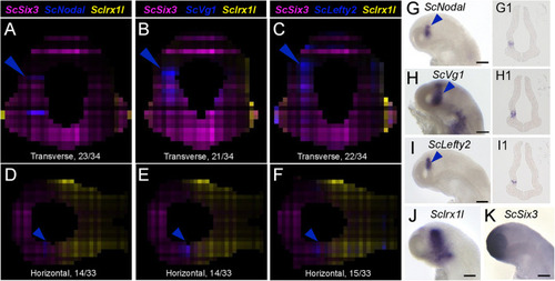
Figure 5. Nodal signaling components exhibit left enriched profiles. (A–F) Digital transverse (A–C) and horizontal (D–F) sections showing merged profiles of ScSix3 (magenta), ScIrx1l (yellow), and in blue ScNodal (A,D), ScVg1 (B,E), ScLefty2 (C,F). Sections are numbered from posterior to anterior in panels (A–C) and from dorsal to ventral in panels (D–F). (G–K) Left lateral views of stage 17 catshark embryonic heads after whole-mount ISH with probes for ScNodal (G), ScVg1 (H), ScLefty2 (I), ScIrx1l (J), and ScSix3 (K). (G1–I1) Horizontal sections of the brain of stage 17 catshark embryos after hybridization with probes for ScNodal (G1), ScVg1 (H1), ScLefty2 (I1). Blue arrowheads point to ScNodal, ScVg1, and ScLefty2 left-restricted digital or ISH signals in the dorsal diencephalon. Scale bars = 200 μm.

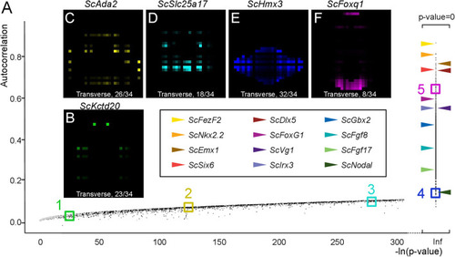
Autocorrelation as an indicator of profile regionalization. (A) Graph showing autocorrelation values (y-axis) and their statistical support [-ln(p-value) on x-axis] for all gene models. Each dot corresponds to a single gene model, in gray if the corresponding total digital expression is below 100, otherwise in black. Gene models with null p-values are shown on the right of the graph with –ln(p-value) = infinite (Inf). Horizontal arrowheads point to dots corresponding to a selection of genes, exhibiting clearly regionalized expressions in ISH experiments. Color codes for these genes are shown boxed in black. Colored boxes delimit sectors of the graph numbered from 1 to 5 and containing gene models with decreasing p-values/increasing autocorrelations (green, sector 1; yellow, sector 2, cyan, sector 3; blue, sector 4; magenta, sector 5). (B–F) Digital transverse sections showing examples of profiles observed in sectors 1 (B), 2 (C), 3 (D), 4 (E), and 5 (F). The corresponding gene identities are indicated and sections are numbered from posterior to anterior.

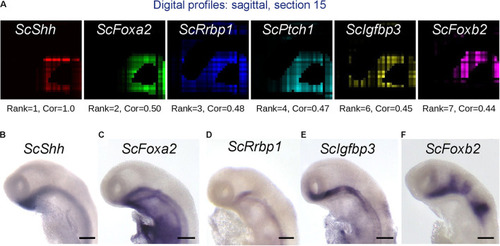
Figure 7. Identification of genes harboring expression correlation with ScShh. (A) Digital profiles on sagittal section number 15 (out of 30, from left to right) of a selection of genes showing a high expression correlation to ScShh (red), ScFoxA2 (green), ScRrbp1 (blue), ScPtch1 (cyan), ScIgfbp3 (yellow), and ScFoxb2 (purple). The rank of each gene in the list of gene models ordered by decreasing correlation to ScShh and the correlation value (Cor) are indicated below each section. (B–F) Left lateral views of stage 17 catshark embryonic heads after ISH using probes for ScShh (B), ScFoxA2 (C), ScRrbp1 (D), ScIgfbp3 (E), and ScFoxb2 (F). Scale bars = 200 μm.