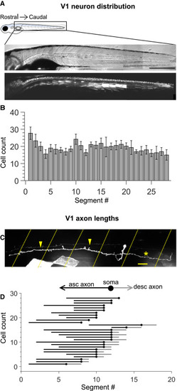
Figure 1. Engrailed⁺ V1 neurons project long, primarily ascending axons

(A) Montaged transmitted light images (top) and confocal images (bottom) of a 5-days post fertilization (dpf) Tg (eng1b:Gal4,UAS:GFP) larva. In this and subsequent figures, rostral is to the left and dorsal to the top. Some non-specific expression of GFP is present in muscle fibers as well. Scale bar, 0.5 mm.

(B) Bar plot showing mean cell count of V1 neurons per segment along the rostro-caudal axis. n = 15 larvae from 4 clutches. Error bars represent SEM.

(C) Representative example of a sparsely labeled V1 neuron in a mid-body segment. Segment borders are shown in yellow dashed lines. Arrowheads mark the ascending axon, and the asterisk marks the descending axon. Scale bar, 20 μm.

(D) Ball and stick plots representing the soma (ball) and ascending and descending axon lengths of V1 neurons (sticks) relative to body segments. n = 28 neurons from N = 18 larvae.

See also Figure S1.

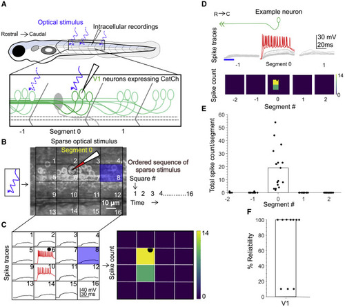
Figure 2. Calibration of V1 spiking evoked by optical stimulus

(A) Schematic of the experimental setup showing targeted intracellular recording and optical stimulation in Tg(eng1b:Gal4,UAS:CatCh) animals.

(B) Schematic of the patterned optical stimulus. A 4 × 4 grid was overlaid on approximately one segment, and each square in the grid (blue square) was optically stimulated in an ordered sequence (right). Position of the recorded cell is shown as a dotted black circle.

(C) Illustration of the analysis. Intracellular recordings elicited from optical stimulation in each grid square (left) are shown. Spiking is denoted in red. Same data are shown as a heatmap and superimposed on the optical stimulus grid (right). Position of the recorded cell is indicated with a black circle.

(D) V1 responses evoked by optical stimuli in segments rostral or caudal to the recorded neuron. Representative traces of activity (top) and spike count (bottom) of the same V1 neuron while the optical stimulation was moved along the rostro-caudal axis are shown. Red traces indicate spiking. Blue bar indicates duration of the optic stimulus.

(E) Quantification of spiking in V1 neurons as the optical stimulus is presented along the rostro-caudal axis. n = 17 neurons. Bar indicates median value.

(F) Reliability of spiking in these neurons with multiple trials of the same optical stimulus. n = 10 neurons. Bar indicates median value.

See also Figure S2.

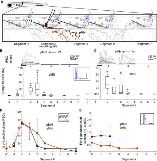
Figure 3. Motor neurons receive input only from local V1 neurons

(A) Schematic of the experimental design showing intracellular recordings from primary (brown) and secondary (orange) motor neurons paired with optical stimulation of V1 neurons (black) along the rostro-caudal axis.

(B) Top: representative overlay of 15 traces of IPSCs recorded in a primary motor neuron (pMN) during illumination of segments 1, 3, and 7 caudal to the recorded neuron soma. Colored trace represents mean. Duration of the optical stimulus is shown as a blue bar. Bottom: boxplots show total charge transfer per segment (inset, illustration) recorded in primary motor neurons. In this and subsequent figures, the box shows the median, 25^th, and 75^th percentile values; whiskers show ±2.7σ. Red asterisks mark segments that were significantly different from noise (p < 0.01). n = 8–26 neurons for each data point.

(C) Same as in (B) for secondary motor neurons (sMNs). n = 10–11 neurons for each data point.

(D and E) Comparison of the percent of squares in the optical stimulus grid that evoked IPSCs (D) and the peak conductance of IPSCs (E) in primary (brown) and secondary (orange) motor neurons. Here and in subsequent figures, circles represent median values and error bars indicate the 25^th and 75^th percentiles. n = 8–26 pMNs and 11 sMNs.

See also Figure S3.

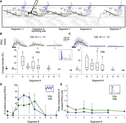
Figure 4. V1 neurons inhibit V2a and V2b neurons locally

(A) Schematic of the experimental design showing intracellular recordings from V2a (green) and V2b (cyan) neurons paired with optical stimulation of V1 neurons (black) along the rostro-caudal axis.

(B) Top: representative overlay of 15 traces of IPSCs recorded in V2a neurons during illumination of segments 1, 3, and 7 caudal to the recorded neuron position. Colored trace represents mean. Duration of the optical stimulus is shown as a blue bar. Bottom: boxplots show the total charge transfer per segment recorded in V2a neurons. Red asterisks mark segments that were significantly different from noise (p < 0.01). n = 8–14 neurons for each data point.

(C) Same as in (B) for V2b neurons. n = 5–9 neurons.

(D and E) Comparison of the percent of squares in the optical stimuli grid that evoked IPSCs (D) and the peak conductance of IPSCs (E) in V2a (green) and V2b (cyan) neurons. n = 8–14 V2as and 5–9 V2bs.

See also Figure S4.

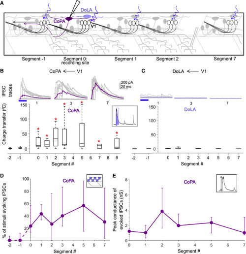
Figure 5. Dorsal horn CoPA neurons receive both local and long-range inputs from V1 neurons

(A) Schematic of the experimental design showing intracellular recordings from CoPA (magenta) and DoLA (violet) neurons paired with optical stimulation of V1 neurons (black) along the rostro-caudal axis.

(B) Top: representative overlay of 15 traces of IPSCs recorded in CoPA neurons during illumination of segments 1, 3, and 7 caudal to the recorded neuron position. Colored trace represents mean. Duration of the optical stimulus is shown as a blue bar. Bottom: boxplots show the total charge transfer per segment recorded in CoPA neurons. Red asterisks mark segments that were significantly different from noise (p < 0.01). n = 7–12 neurons for each data point.

(C) Same as in (B) for DoLA neurons. n = 4–5 neurons for each point.

(D and E) Comparison of the percent of squares in the optical stimuli grid that evoked IPSCs (D) and the peak conductance of IPSCs (E) in CoPA neurons. n = 7–12 neurons.

See also Figure S5.

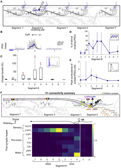
Figure 6. Local V1 synapses onto CoPr neurons and normalized connectivity map

(A) Schematic of the experimental design showing intracellular recording from CoPr neurons (blue) paired with optical stimulation of V1 neurons (black) along the rostro-caudal axis.

(B and C) Representative traces of IPSCs (B) and the total charge transfer (C) recorded in CoPr neurons with optical stimulation of V1 neurons along different segments in the rostro-caudal axis. Colored traces in (B) indicate mean. Red asterisks mark segments that were significantly different from noise (p < 0.05).

(D and E) Comparison of the percent of squares in the optical stimuli grid that evoked IPSCs (D) and the conductance of IPSCs (E) in CoPr neurons. n = 5–7 neurons for each point.

(F) Summary of V1 connectivity to different post-synaptic targets. Top: schematic of the inferred connectivity of V1 neurons (black) to different targets locally and distally is shown. Yellow dots symbolize inhibitory synapses. Bottom: heatmap shows normalized charge transfer for the different post-synaptic targets along the rostro-caudal axis. The charge transfer per segment for each recorded neuronal target was normalized to its measured intrinsic neuronal conductance (inverse of R_in). Median values of normalized charge transfer for each target cell population are plotted. Values for segment 4 and segment 6 were interpolated as averages of the two neighboring segments. The resulting values are plotted on the same color scale for all target populations.

See also Figure S6.

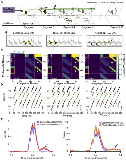
Figure 7. Modeling spinal circuitry with local and distal V1 inhibition

(A) Schematic of the computational model showing a reduced V1 (black), V2a (green), and motor neuron (MN) (brown) network driven by rostrally located pacemaker neurons (purple box).

(B) Schematic of 3 different network structures simulated with the network model. Left: local connectivity from V1 neurons onto MNs and V2as. V1s synapse onto V2as and MNs located within 1–3 segments. Middle: distal connectivity from V1s onto MNs and V2as. V1s synapse onto V2as and MNs located 4–6 segments away. Right: mixed local-distal connectivity from V1s. V1s synapse onto MNs located 4–6 segments away and V2as located within 1–3 segments.

(C) Heatmap showing connectivity weights for neurons across 3 different network models. Connections outlined in yellow are gap junctional and follow a logarithmic scale. Asterisks indicate connection weights that are altered across models.

(D) Raster plots of spike times from 1 representative simulation of each network.

(E) Spiking of MNs with respect to a normalized swim cycle. Black arrow points to the extraneous spiking observed for both distal MN/distal V2a connectivity (left) and more weakly in distal MNs/local V2a connectivity (right).

See also Figure S7 and Tables S1 and S2.