
- Title
-
ACME: Automated Cell Morphology Extractor for Comprehensive Reconstruction of Cell Membranes
- Authors
- Mosaliganti, K.R., Noche, R.R., Xiong, F., Swinburne, I.A., and Megason, S.G.
- Source
- Full text @ PLoS Comput. Biol.
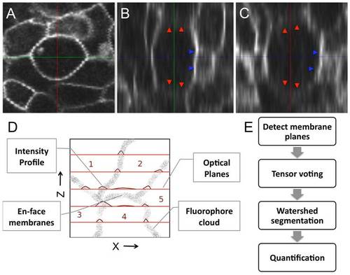
Reconstructing the membrane signal by eliminating intensity inhomogeneities. A single cell membrane is shown across (A), (B), and (C) sections. The plane shows a consistently bold and uniform membrane signal while the and views show a non-uniform membrane signal. Membrane planes en-face to the optical planes (marked by red arrows) are very weak and markedly diffuse in intensity. Membranes orthogonal to the imaging plane are sharper (blue arrows). (D) A qualitative model describing the formation of a membrane image under a fluorescent microscope. Flourophores tagged to membranes are shown as a point cloud (input). The focal planes are shown in red and the obtained intensity profiles on the plane are shown as plots. Cell membranes imaged oblique and en face such as the interface between cells are poorly visible in comparison to those orthogonal to the focal planes. (E) Three stages in the reconstruction process: (i) Detect membrane planes by mining for planar fluorophore distributions. This allows even weak membranes (en-face or oblique) to be extracted and accounts for intensity inhomogeneity. (ii) Voting to fill structural gaps or holes in the membrane signal that may not be contiguous. (iii) Region segmentation using the watershed algorithm to extract three-dimensional cell meshes for quantification. |
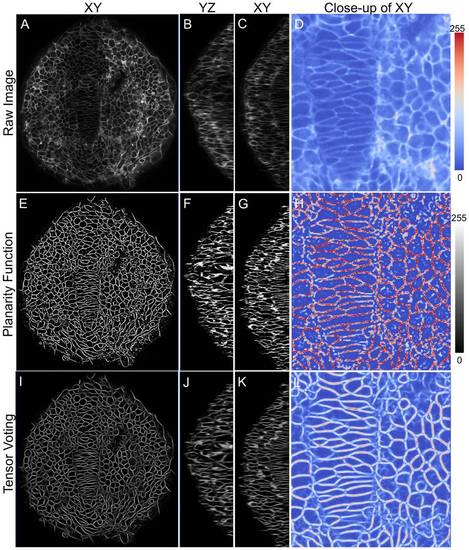
High-fidelity reconstruction of zebrafish membrane images. Significant improvement in membrane signal quality is shown in XY, XZ and YZ planes. (A-D) Raw data showing dorsal view (anterior on top) of zebrafish neuroepithelium (ne) and notochord at 12 hpf, (E-H) Planarity function intermediate output and (I-L) Tensor voting final output. The last image in each panel shows a color-mapped zoomed view for easy comparison. |
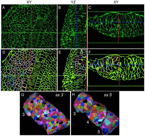
Robust reconstruction and segmentation of cells in the presomitic mesoderm. (A-C) Raw image data showing presomitic mesoderm on 2D image planes (XY,YZ, and XZ) at 3ss. (D-F) Segmentation meshes overlaid on reconstructed membrane images demonstrate excellent localization. Each mesh was randomly colored for visually separating adjacent cells easily. (G,H) 3D rendering of membrane segmentations at 3ss and 5ss. Somites 3, 4 and 5 at 5ss are formed from the presomitic tissue at 3ss by cell sorting and rearrangement. |
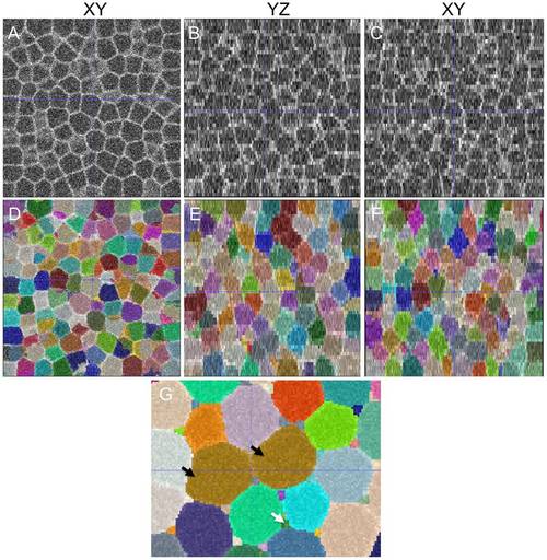
Accurate and highly-sensitive algorithm performance on synthesized 3D membrane images. (A-C) Synthesized cell structures in 3D along XY, YZ and XZ sections with image noise added (Table 2). As in the case of real-world images, the lateral resolution significantly differs from the axial resolution. (D-F) Segmentations overlaid on the raw image with a 50% opacity function. (G) An example of under-segmentation (brown cells, black arrows) and over-segmentation (interstitial fragments, white arrows) in the image. The errors could be filtered out by size criteria. |
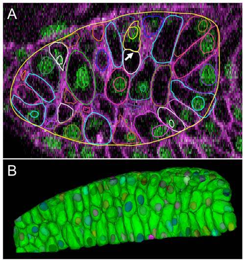
Robust correspondence between membrane and nuclear segmentations. Algorithm performance was assessed by matching automated segmentations obtained from the nuclear and membrane channels. In the ideal case, each individual nucleus would match with a unique membrane and vice-versa. (A) A single 2D image plane is shown with contours of membrane and nuclear segmentations overlaid on raw data. Some cells have their corresponding nuclei located out-of-plane. The lack of a one-to-one correspondence indicates an error. For example, an over-segmentation of the membrane channel (white arrow) causes one of the membrane components to not contain a nucleus. (B) 3D renderings of cells from membrane and nuclear segmentations. EXPRESSION / LABELING:
|
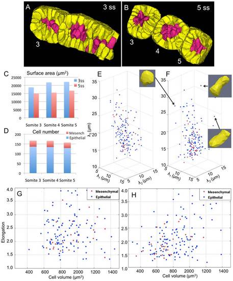
Algorithm-enabled quantification of cell dynamics during somite formation. Retrospective cell tracing of epithelial (yellow) and mesenchymal (red) cells from formed somites at (B) 5ss back to the presomitic mesoderm at (A) 3ss. (C) Corresponding decrease in somite tissue surface area during the formation of somites 3, 4, and 5. (D) Epithelial and mesenchymal cell numbers in respective somites at 5ss. (E,F) Three-dimensional cell shape quantified by the length of their principal axes at 3ss and 5ss. (G,H) Scatter plots of elongation (2λ3/λ1+λ2) and cell volumes at 3ss and 5ss. The two cell populations show different behavior. Statistical analysis of the two distributions show that mesenchymal cells (red) tend to cluster, round-up, and shrink in size on average. |

Tensor voting field determination. (A) 2D voting field parameters. (B) Heat map showing the stick voting field saliencies in 2D. The stick tensor is represented using line glyphs and overlaid on the figure. (C) A simple example showing two sampled intersecting circles and their reconstruction (D). |
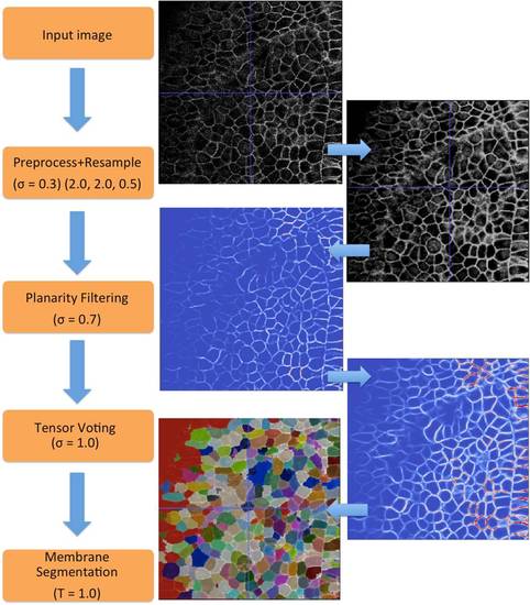
A flowchart of processing filters and parameters with intermediate outputs. There are four filters that take the input image to produce an output segmented image. For each step on the left, the corresponding input and output image is shown on the right. |
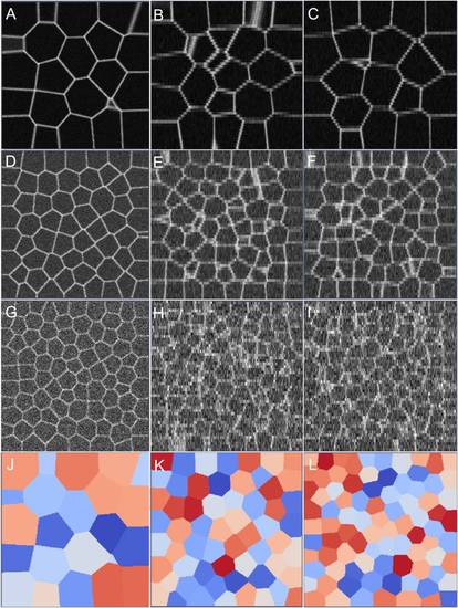
Synthetic membrane images along XY, XZ, and YZ sections. The (σ, λ) values were sampled as (A-C) (0.01, 1.00), (D-F) (0.05, 0.6), and (G-I) (0.1, 0.1). Corresponding ground truth segmentation images (XY) are shown in (J-L). |