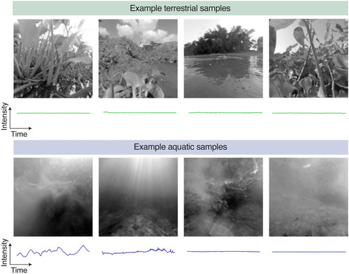
Examples of the first frame and the average change in intensity over time from the terrestrial and aquatic video samples. Each image shows the green (G) channel of one sample's first frame. The images are shown as log light intensity for visibility. Below each image is the average intensity as a function of time for the same sample. For all temporal plots, the abscissa is time with a span of 10 s, and the ordinate is intensity on an arbitrary scale.

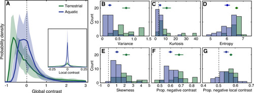
Contrast distributions differed between the terrestrial and aquatic samples. (A) Solid lines show the mean probability density of global contrast in terrestrial (green) and aquatic (blue) samples. The shaded area indicates the region plus or minus one standard deviation of the mean. (B–G) Statistics of the contrast distributions for each environment are plotted as histograms, including the variance (B), kurtosis (C), entropy (D), skewness (E), proportion negative global contrast (F) and proportion negative local contrast based on the difference of Gaussians contrast operator (G). Symbols above indicate the mean and standard deviation. Dashed lines indicate kurtosis = 3 (Gaussian), skewness = 0 (symmetric) and proportion negative contrast = 0.5. The inset in panel (A) shows the distribution of local contrast, which is much broader for the terrestrial samples. Note that the mean global contrast is always effectively zero because contrast is defined relative to the mean intensity of each sample, and is thus not included in the plots.

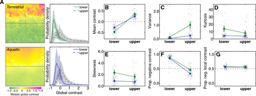
Contrast distributions differ in the upper and lower visual fields of both environments. (A) Heatmaps show the median contrast across the visual field for the terrestrial (upper) and aquatic (lower) samples. Line plots show the average probability density of contrast in the upper and lower visual fields. Shaded regions indicate plus or minus one standard deviation of the mean. (B–E) Statistics of the contrast distributions, including the mean (B), variance (C), kurtosis (D), skewness (E), proportion negative global contrast (F) and proportion negative contrast based on the difference of Gaussians local contrast operator (G). Values for individual samples are plotted as smaller circles; mean and 95% confidence intervals are plotted as large circles and vertical lines.

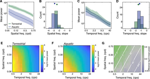
Spatiotemporal power spectra indicate more fast speeds in the aquatic samples. (A) Spatial power spectra. Lines indicate the mean log power across samples and shaded regions indicate plus or minus one standard deviation. Green and blue colors indicate terrestrial and aquatic samples, respectively. Cpd denotes cycles/degree. (B) Histograms of the best fit slopes of spatial power spectra in (A). The markers and errorbars show the means and the 95% confidence intervals. (C) Temporal power spectra, plotted in the same manner as (A). Cps denotes cycles/second. (D) Histograms of the best fit slope of temporal power spectra in (C). (E) The median terrestrial spatiotemporal power spectrum. (F) The median aquatic spatiotemporal power spectrum. (G) The difference between logarithmic values in (E) and (F). Lines illustrate iso-speed contours derived from the ratio of temporal frequency and spatial frequency.

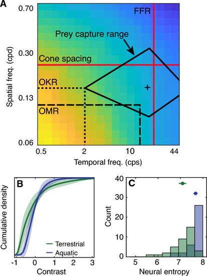
Implications for understanding visually guided behavior and neural coding. (A) The colormap shows the spatiotemporal power spectrum of the aquatic samples, reproduced from Fig. 4F using the same color scale. The horizontal dotted and dashed lines represent the spatial limit (visual acuity) of the optokinetic response (OKR) in larvae (0.16 cpd)²¹ and the optomotor response (OMR) in larvae (0.11 cpd, see our estimation based on²² in the methods section), respectively. The vertical dotted and dashed lines represent the approximate temporal limit of the OKR (~ 2 cps depending on stimulus velocity²⁰) and the OMR (~ 14 cps^18,19), respectively. Note that the temporal limit depends on the tested spatial frequencies and velocities. The solid black lines indicate the spatial and temporal stimulus bounds for larval prey capture (spatial: 0.09 to 0.33 cpd; temporal: 2 cps to 60 cps) and the cross indicates the "ideal" prey stimulus²⁵. The red lines indicate the flicker fusion rate (FFR; 20 Hz)^26,27 and the theoretical cone spacing limit (0.24 cpd) for larvae²¹. (B) Cumulative probability distributions for visual contrast are shown to illustrate different optimal neural response nonlinearities as described in³². (C) We applied each of the nonlinearities from (B) to the aquatic imagery in our dataset and computed the entropy of the predicted neural responses.