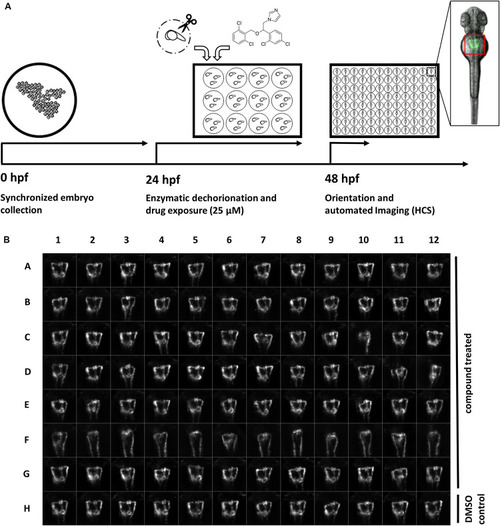
A screening workflow to score potential nephrotoxicity of approved drugs. (A) Schematic illustration of the drug toxicity screening pipeline. Synchronized embryos were obtained by collecting eggs from batch and pairwise crossings within a maximum interval of 30 min. At 24 h post fertilization (hpf) green fluorescent protein (GFP) positive embryos were enzymatically dechorionated using pronase and 20 embryos were transferred in each well of a 12-well plate. Different compounds were added to each well to a final concentration of 25 μM. At 48 hpf, and after 24 h drug exposure, embryos were washed, transferred into agarose filled microtiter plates, oriented within cavities generated with 3D-printed orientation tools and automatically imaged. The location of embryonic kidneys within image data was automatically determined using center of mass detection after thresholding of maximum z-projections. Center of mass coordinates were used to automatically crop maximum z-projections to thumbnails images with 257 × 257 pixels dimension [see also (B)]. Thumbnail images were used for all subsequent analysis steps. (B) Representative example of montage of pronephros thumbnail images, which was generated for each experimental 96-well plate. Each row was loaded with differently treated embryos. Row A-G show compound treated embryos, row F shows embryos with severely altered pronephros morphology, and row H shows embryos treated only with DMSO serving as plate internal negative controls. Permission to reuse and Copyright: It is made available under a CC-BY-ND 4.0 International license.

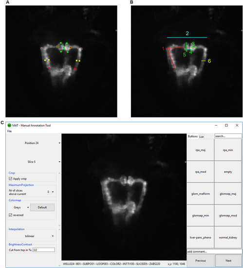
Analysis and annotation of pronephric phenotypes. (A,B) Quantitative measuring of morphological phenotypes of pronephroi. (A) Positions of 16 reference points are indicated that were manually assigned to each pronephros thumbnail image. (B) Illustration of calculated morphological parameters based on reference points in (A). Colors in (A,B) indicate which reference points in panel (A) were used for the calculation of morphological features in panel (B): (1) pronephric angle (only left side is shown – angleL), (2) tubular distance (tubDist), (3) glomerular height (only right side is shown – glomHeightR), (4) glomerular separation (glomSep), (5) glomerular width (only left side is shown – glomWidthL), and (6) tubular diameter (only right side is shown – tubDiamR). (C) Screenshot of software tool for manual annotation of large image datasets (https://doi.org/10.5281/zenodo.3367365). The manual annotation tool allows to browse, filter, auto-center, visualize and annotate complex multidimensional image datasets in an intuitive and blinded manner without any additional data pre-processing steps. In this study, the tool was used to assign up to 10 phenotypic categories to each acquired embryonic pronephros. Abbreviations: reduced pronephros angle major (rpa_maj), reduced pronephros angle minor (rpa_min), reduced pronephros angle moderate (rpa_mod), glomerular malformation (glom_malform), glomerular separation major (glomsep_maj), glomerular separation minor (glomsep_min), glomerular separation moderate (glomsep_mod), impaired liver pancreas area (liver-panc_pheno) and normal kidney (normal_kidney). Permission to reuse and Copyright: It is made available under a CC-BY-ND 4.0 International license.

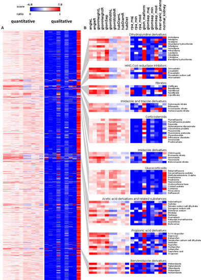
Overview of scored quantitative morphometric parameters and qualitative manual annotations. (A) Heat map visualizations illustrating the pronephric phenotypic alterations upon compound treatment for each assayed compound. Heat maps are sorted according to the D-level of the Anatomical Therapeutic Chemical (ATC) Classification System (for fully labeled heat maps please refer to Supplementary Figures S3, S4). The left panel shows quantitative parameters shown as color-coded z-score. Shown are z-score changes of pronephric angle left (angleL), pronephric angle right (angleR), glomerular height left (glomHeightL), glomerular height right (glomHeightR), glomerular separation (glomSep), glomerular width left (glomWidthL), glomerular width right (glomWidthR), tubular diameter left (tubDiamL), tubular diameter right (tubDiamR) and tubular distance (tubDist). See also labelling of heat map columns in panel (B). The right panel shows qualitative annotations as a ratio of embryos assigned with a certain category. Legend indicates colors assigned to values. Shown are ratios for reduced pronephros angle major (rpa_maj), reduced pronephros angle minor (rpa_min), reduced pronephros angle moderate (rpa_mod), glomerular malformation (glom_malform), glomerular separation major (glomsep_maj), glomerular separation minor (glomsep_min), glomerular separation moderate (glomsep_mod), impaired liver pancreas area (liver-panc_pheno) and normal kidney (normal_kidney). See also labeling of heat map columns in panel (B). (B) Magnified view on illustrative examples of compound classes enriched with substances causing pronephric phenotypes. Permission to reuse and Copyright: It is made available under a CC-BY-ND 4.0 International license.

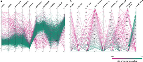
Distribution of phenotypic features upon compound treatment. Parallel coordinates plot visualizations showing the distribution of phenotypic features of pronephroi upon compound treatment. Each line plot represents a single compound treatment. In total, 1237 compound treatments are shown. The color of lines indicates the ratio of embryos within one treatment group scored as “normal_kidney” using manual annotation (from 0% (magenta, all abnormal) to 100% (green, all normal)). Y-axes show the (A) mean fold change for different quantitative morphometric parameters, or (B) ratio of embryos assigned with qualitative manual annotations. Abbreviations as in Figure 3. Permission to reuse and Copyright: It is made available under a CC-BY-ND 4.0 International license.

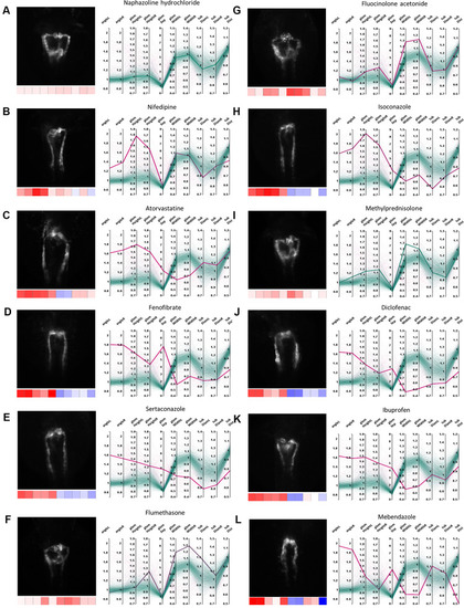
Examples of pronephric phenotypes. Illustrative examples of drug induced phenotypic changes for several compound classes. For each compound a thumbnail image, a heat map z-score visualization (below thumbnail) and a parallel coordinates plot of fold changes of quantitative morphological features are shown. In the parallel coordinates plots, thick lines indicate the shown compound and thin lines represent all other compound treatments; color codes as in Figures 3, 4. (A) Naphazoline hydrochloride (class, sympathomimetics); showing no effect (please see Supplementary Figure S5 for DMSO-only control), (B) nifedipine (class, dihydropyridine derivatives), (C) atorvastatine (class, HMG CoA reductase inhibitors), (D) fenofibrate (class, fibrates), (E) sertaconazole (class, imidazole and triazole derivatives), (F) flumethasone (class, corticosteroids, moderately potent (group II)), (G) fluocinolone acetonide (class, corticosteroids, potent (group III)), (H) isoconazole (class, imidazole derivatives), (I) methylprednisolone (class, glucocorticoids), (J) diclofenac (class, acetic acid derivatives and related substances), (K) ibuprofen (class, propionic acid derivatives), and (L) mebendazole (class, benzimidazole derivatives). Permission to reuse and Copyright: It is made available under a CC-BY-ND 4.0 International license.

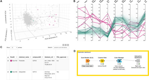
Exploring and browsing the generated zebrafish embryo nephrotoxicity dataset. Shown are screenshots of an interactive exploration tool generated using KNIME (see Supplementary Software S4). The workflow allows to visualize the full result table as well as a PCA scatter plot and a parallel coordinates line plot of the quantitative features in a single HTML window. The tool allows highlighting single compounds, compound groups or classes by selecting single lines in a parallel coordinates plot, sliders for limiting PCA range (not shown) or through searching in the data result table. Selected results are shown as colored dots in the PCA scatterplot, thicker lines in the parallel coordinates plot or as filtered rows in the results table. In this figure all panels show highlighted results for the propionic acid derivatives compound class. (A) PCA plot, (B) parallel coordinate plot, (C) result table. Color code for highlighted dots, lines or rows in panel (A–C) as in Figures 3, 4 with 0% (magenta, all abnormal) to 100% (green, all normal). (D) KNIME workflow generating the interactive tool. A video tutorial is available at https://youtu.be/A4Eqe1Aju4A. Permission to reuse and Copyright: It is made available under a CC-BY-ND 4.0 International license.