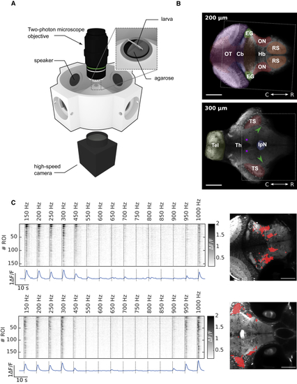
Experimental Setup for Acoustic Stimulation and Simultaneous Recording of Neural Activity and Behavior

(A) Zebrafish larvae were head restrained in a drop of low-melting-point agarose inside a 3D-printed recording chamber. Acoustic stimulations (pure tones at different frequencies) were delivered using waterproof speakers. Spontaneous and evoked neuronal activity was monitored by two-photon calcium imaging while movements of the tail were simultaneously recorded with a high-speed camera.

(B) Two optical sections of a larva’s brain pan-neuronally expressing GCaMP5 (Huc:GCaMP5). Cb, cerebellum; EG, eminentia granularis; Hb, hindbrain; IpN, interpeduncular nucleus; ON, octaval nuclei; OT, optic tectum; RS, reticulospinal neurons; Th, thalamus; Tel, telencephalon; TS, torus semicircularis. Green arrowheads, lateral longitudinal fascicle; purple asterisks, nucleus of the medial longitudinal fascicle. Scale bars, 100 μm. Dotted rectangles correspond to area displayed in (C).

(C) Two examples of sensory activity in the octaval nuclei (top) and torus semicircularis (bottom). Top: raster example for one larva averaged across trials for each stimulus frequency is shown. Bottom: activity averaged across ROIs is shown. Right: topography of ROIs selected as responsive using linear regression corresponding to the rasters on the left is shown. Scale bar, 100 μm. See also Figures S1 and S2.

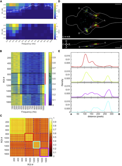
Spatially Distinct Clusters Represent Low- and High-Frequency Information

(A) Top: average audiogram (5 larvae at 8 dpf), measured as the amplitude of the neuronal response fit by a linear regression model, averaged over all ROIs in the brain. White curve: average threshold and SEM are shown. Bottom: single larva example is shown.

(B) Frequency tuning curves for 13 larvae at 8 dpf, grouped in 4 clusters using k-means clustering algorithm with Euclidean distance on normalized ΔF/F values. Different larvae were imaged at different optical sections. Clusters 1–4 are represented in red, green, cyan, and magenta.

(C) Similarity matrix based on the Euclidean distance for the clusters in (B).

(D) Spatial distribution of the 4 clusters presented in (B). All 13 larvae were aligned on a reference stack using affine transformation. Top: maximum density projection across the Z axis is shown. Bottom: maximum density projection across the y axis is shown. Scale bar, 100 μm.

(E) Spatial density of ROIs for each cluster along the gray dashed AB axis in (D), averaged across both hemispheres. See also Figures S4 and S5.

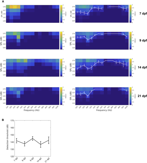
Audiograms at Different Development Stages

(A) Right: average audiogram at 7 dpf (4 larvae), 9 dpf (7 larvae), 14 dpf (3 larvae), and 21 dpf (5 larvae) measured as the amplitude of the neuronal response fit by a linear regression model, averaged over all ROIs in the brain. White curve: average threshold and SEM are shown. Left: single larva example is shown.

(B) Detection threshold, the lowest amplitude at which a neuronal response was detected, averaged across larvae during the different developmental stages (mean ± SEM). Means at different ages were not significantly different (p = 0.4381; one-way ANOVA). See also Figure S3.

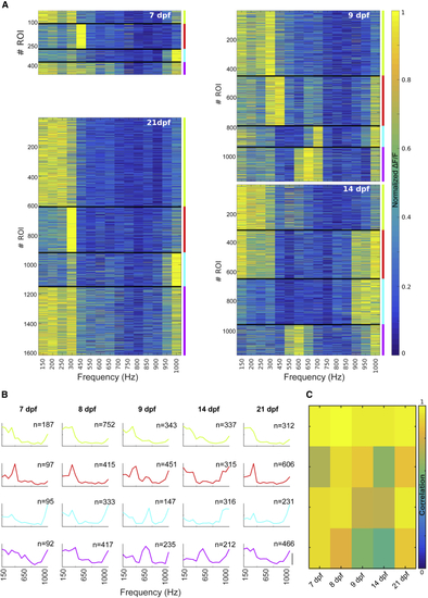
Frequency Tuning Curves at Different Developmental Stages

(A) Frequency tuning curves grouped in 4 clusters using k-means clustering algorithm at 7 dpf (6 larvae), 9 dpf (11 larvae), 14 dpf (3 larvae), and 21 dpf (5 larvae).

(B) Average normalized tuning curves across ROIs grouped in 4 clusters throughout the larva’s development, from 7 to 21 dpf. Similar tuning curves were assigned to the same cluster across developmental stages by maximizing the correlation between the tuning curves and the average tuning across ages. Scale bar, 0.5 ΔF/F. The colors represent the clusters indicated in (A). Top right corner: the number of ROIs per cluster is shown.

(C) Correlation matrix used to order the clusters in (B). We correlated the tuning curve for each cluster at each developmental stage with the average tuning curve across ages. All possible permutations of cluster assignments were tested. The matrix shows the solution that maximized the average correlation. Average correlation: 0.85 ± 0.14 (SD).

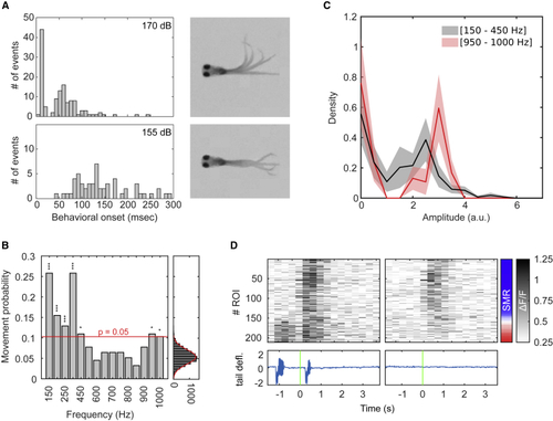
Auditory-Induced Tail Motor Behaviors

(A) Delay histogram between the onset of auditory stimulation and the onset of tail movements (7 larvae) Top: auditory stimulation using 170 dB re 1 μPa stimuli resulted in a bimodal distribution probably representing short latency C-starts and long-latency C-starts. Bottom: auditory stimulation using 155 dB re 1 μPa stimuli resulted in a distribution of longer and more variable latencies.

(B) Probability of having at least one tail bout in a 500-ms time window after stimulus onset for each frequency. A null model was created by generating data following the same inter-bouts interval distribution as the experimental data (left). p values were computed using the null model distribution and subsequently adjusted using Bonferroni correction. Red dashed line, significance threshold for α = 0.05 after Bonferroni correction. n = 10 larvae.

(C) Average density distribution (mean ± SEM) of bout amplitudes (10 larvae), elicited by low-frequency stimuli (150 Hz and 450 Hz; 134 bouts) in black and high-frequency stimuli (950 Hz and 1,000 Hz; 30 bouts) in red. The amplitude of a tail bout was defined as the maximum curvature during the bout. The medians of the two distributions were not significantly different (p = 0.73; two-sided rank-sum test).

(D) Top: single trial raster on a single larva. ROIs are ordered by their sensorimotor ratio, computed as (R²_mvt − R²_stim)/(R²_mvt + R²_stim). The sensorimotor ratio ranges from −1 (sensory ROIs, in blue) to +1 (behavior-related ROIs, in red). Bottom: tail deflection is shown, green bar, auditory stimulus onset.

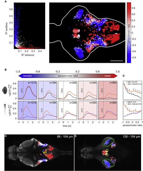
Sensorimotor Properties of the Auditory Neural Circuit

(A) Left: distribution of ROIs R² values for movement and behavior with the corresponding sensorimotor ratio value. Right: topography of ROI’s sensorimotor ratio for 10 larvae at 8 dpf is shown. Scale bar, 100 μm.

(B) Top: average ΔF/F over ROIs after an auditory stimulation around auditory stimulus onset (t = 0 s) for ROIs grouped in 5 bins according to their sensorimotor ratio. Stimulus frequencies from 150 to 450 Hz were pooled together. Orange curve, stimulus followed by a tail movement within a 500-ms time window after stimulus onset. Black curve, stimulus not followed by a tail movement. Bottom: average ΔF/F across ROIs when the fish moved is shown (t = 0 s: movement onset). Orange curve, tail movement preceded by an auditory stimulation. Purple curve, self-generated movement. In the bottom panels, the delay between the orange curve (stimulus-induced movement) and the purple curve (self-generated movement) corresponds to sensory processing, because the stimulus occurs before the movements.

(C) Average peak ΔF/F value (mean ± SEM) across ROIs around auditory stimulus onset (top panel) or tail movement onset (bottom panel). ROIs were binned into 10 groups based on their sensorimotor ratio value. Bins were compared using the two-tailed Wilcoxon rank sum test, and p values were subsequently adjusted using Bonferroni correction.

(D) The topography of the sensorimotor ratio (blue, sensory; white, sensorimotor; red, motor), superimposed to the Elavl3-GCaMP5 line in the z-brain atlas. Yellow, facial motor and octavolateralis efferent; on, octaval nuclei; rs, reticulospinal circuits. Top right corner: depth of the imaged plane is shown.

(E) The topography of the sensorimotor ratio over the Elavl3-GCaMP5 line in the z-brain atlas. Green, torus semicircularis; yellow, nucleus of the medial longitudinal fascicle; orange, cerebellar vglut2-enriched area. Top right corner: depth of the imaged plane is shown. See also Figure S6 and Videos S1 and S2.

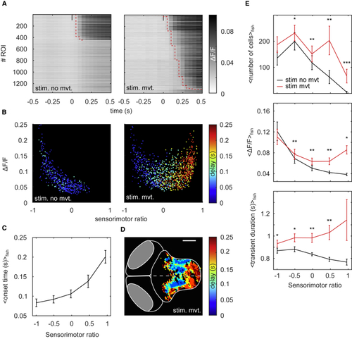
Increased Network Activity and Duration of Calcium Transients Mediates Sensorimotor Transformation

(A) Example rasters of a single larva averaged over trials for which auditory stimuli induced (stim. mvt.) or did not induce a tail movement (stim. no mvt.). ROIs are sorted by the onset time of their calcium transients. Red dotted line, transient onset. Transient onset was estimated only for ROIs whose activity after stimulation was 2 SDs above their mean activity before stimulation (activity baseline).

(B) Example of ΔF/F as a function of sensorimotor ratio; colormap, onset time of the calcium transients.

(C) Onset time (mean ± SEM) as a function of sensorimotor ratio for 27 larvae. ROIs were binned into 5 groups based on their sensorimotor ratio.

(D) Topography of the onset time for the same larva as in (A) and (B). Scale bar, 100 μm.

(E) Top: number of ROIs above the 3 SD threshold for each sensorimotor ratio bin (mean ± SEM). Middle: peak ΔF/F for each bin is shown (mean ± SEM). Bottom: transient duration computed as the full width at half maximum of the calcium transients for each bin is shown (mean ± SEM). Red line, auditory stimulation followed by a tail movement in a 500-ms time window after stimulation onset. Black line, auditory stimulation not followed by a tail movement. Results were pooled across 27 larvae. Bins were compared using the one-tailed Wilcoxon paired signed rank test, and p values were subsequently adjusted using Bonferroni correction. See also Figure S7.