ZFIN All Figures, van der Plas <i>et al.</i>, 2023

Figure 1

cRBMs construct Hidden Units by grouping neurons into assemblies.

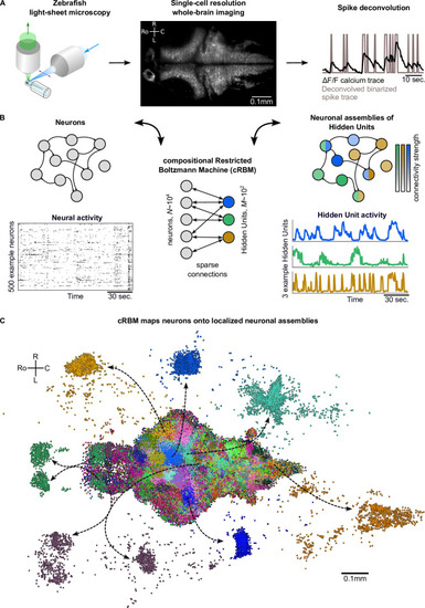
(A) The neural activity of zebrafish larvae was imaged using light-sheet microscopy (left), which resulted in brain-scale, single-cell resolution data sets (middle, microscopy image of a single plane shown for fish #1). Calcium activity $Δ F / F$ $Δ F / F$ was deconvolved to binarized spike traces for each segmented cell (right, example neuron). (B) cRBM sparsely connects neurons (left) to Hidden Units (HUs, right). The neurons that connect to a given HU (and thus belong to the associated assembly), are depicted by the corresponding color labeling (right panel). Data sets typically consist of $N \sim 10^{4}$ $N \sim 10^{4}$ neurons and $M \sim 10^{2}$ $M \sim 10^{2}$ HUs. The activity of 500 randomly chosen example neurons (raster plot, left) and HUs 99, 26, 115 (activity traces, right) of the same time excerpt is shown. HU activity is continuous and is determined by transforming the neural activity of its assembly. (C) The neural assemblies of an example data set (fish #3) are shown by coloring each neuron according to its strongest-connecting HU. 7 assemblies are highlighted (starting rostrally at the green forebrain assembly, going clockwise: HU 177, 187, 7, 156, 124, 64, 178), by showing their neurons with a connection $| w | \geq 0.1$ $| w | \geq 0.1$ . See Figure 3 for more anatomical details of assemblies. R: Right, L: Left, Ro: Rostral, C: Caudal.

Figure 2

cRBM is optimized to accurately replicate data statistics.

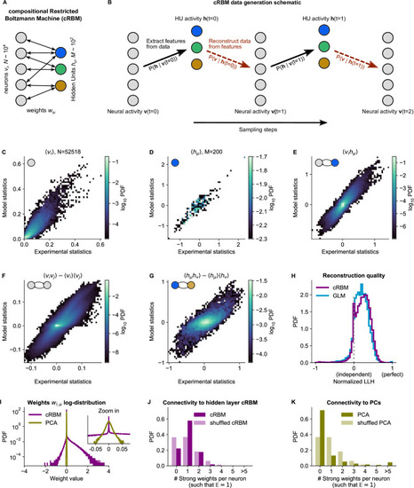
(A) Schematic of the cRBM architecture, with neurons $v_{i}$ $v_{i}$ on the left, HUs $h_{μ}$ $h_{μ}$ on the right, connected by weights $w_{i, μ}$ $w_{i, μ}$ . (B) Schematic depicting how cRBMs generate new data. The HU activity $h (t)$ $h (t)$ is sampled from the visible unit (i.e. neuron) configuration $v (t)$ $v (t)$ , after which the new visible unit configuration $v (t + 1)$ $v (t + 1)$ is sampled and so forth. (C) cRBM-predicted and experimental mean neural activity $⟨ v_{i} ⟩$ $⟨ v_{i} ⟩$ were highly correlated (Pearson correlation $r_{P} = 0.91$ $r_{P} = 0.91$ , $P < 10^{- 307}$ $P < 10^{- 307}$ ) and had low error ( ${nRMSE}_{⟨ v_{i} ⟩} = 0.11$ ${nRMSE}_{⟨ v_{i} ⟩} = 0.11$ , normalized Root Mean Square Error, see Materials and methods - ‘Calculating the normalized Root Mean Square Error’ ). Data displayed as 2D probability density function (PDF), scaled logarithmically (base 10). (D) cRBM-predicted and experimental mean Hidden Unit (HU) activity $⟨ h_{μ} ⟩$ $⟨ h_{μ} ⟩$ also correlated very strongly ( $r_{P} = 0.93$ $r_{P} = 0.93$ , $P < 10^{- 86}$ $P < 10^{- 86}$ ) and had low ${nRMSE}_{⟨ h_{μ} ⟩} = 0.15$ ${nRMSE}_{⟨ h_{μ} ⟩} = 0.15$ (other details as in C) (E) cRBM-predicted and experimental average pairwise neuron-HU interactions $⟨ v_{i} h_{μ} ⟩$ $⟨ v_{i} h_{μ} ⟩$ correlated strongly ( $r_{P} = 0.74$ $r_{P} = 0.74$ , $P < 10^{- 307}$ $P < 10^{- 307}$ ) and had a low error ( ${nRMSE}_{⟨ v_{i} h_{μ} ⟩} = 0.09$ ${nRMSE}_{⟨ v_{i} h_{μ} ⟩} = 0.09$ ). (F) cRBM-predicted and experimental average pairwise neuron-neuron interactions $⟨ v_{i} v_{j} ⟩$ $⟨ v_{i} v_{j} ⟩$ correlated well ( $r_{P} = 0.58$ $r_{P} = 0.58$ , $P < 10^{- 307}$ $P < 10^{- 307}$ ) and had a low error ( ${nRMSE}_{⟨ v_{i} v_{j} ⟩} = - 0.09$ ${nRMSE}_{⟨ v_{i} v_{j} ⟩} = - 0.09$ , where the negative nRMSE value means that cRBM-predictions match the test data slightly better than the train data). Pairwise interactions were corrected for naive correlations due to their mean activity by subtracting $⟨ v_{i} ⟩ ⟨ v_{j} ⟩$ $⟨ v_{i} ⟩ ⟨ v_{j} ⟩$ . (G) cRBM-predicted and experimental average pairwise HU-HU interactions $⟨ h_{μ} h_{ν} ⟩$ $⟨ h_{μ} h_{ν} ⟩$ correlated strongly ( $r_{P} = 0.73$ $r_{P} = 0.73$ , $P < 10^{- 307}$ $P < 10^{- 307}$ ) and had a low error ( ${nRMSE}_{⟨ h_{μ} h_{ν} ⟩} = 0.17$ ${nRMSE}_{⟨ h_{μ} h_{ν} ⟩} = 0.17$ ). (H) The low-dimensional cRBM bottleneck reconstructs most neurons above chance level (purple), quantified by the normalized log-likelihood (nLLH) between neural test data v_i and the reconstruction after being transformed to HU activity (see Materials and methods - ‘Reconstruction quality’). Median normalized = ${nLLH}_{cRBM}$ ${nLLH}_{cRBM}$ 0.24. Reconstruction quality was also determined for a fully connected Generalized Linear Model (GLM) that attempted to reconstruct the activity of a neuron v_i using all other neurons $v_{- i}$ $v_{- i}$ (see Materials and methods - ‘Generalized Linear Model’). The distribution of 5000 randomly chosen neurons is shown (blue), with median ${nLLH}_{GLM} = 0.20$ ${nLLH}_{GLM} = 0.20$ . The cRBM distribution is stochastically greater than the GLM distribution (one-sided Mann Whitney U test, $P < 10^{- 42}$ $P < 10^{- 42}$ ). (I) cRBM (purple) had a sparse weight distribution, but exhibited a greater proportion of large weights $w_{i, μ}$ $w_{i, μ}$ than PCA (yellow), both for positive and negative weights, displayed in log-probability. (J) Distribution of above-threshold absolute weights $| w_{i, μ} |$ $| w_{i, μ} |$ per neuron v_i (dark purple), indicating that more neurons strongly connect to the cRBM hidden layer than expected by shuffling the weight matrix of the same cRBM (light purple). The threshold $Θ$ $Θ$ was set such that the expected number of above-threshold weights per neuron $E (# w_{i} > Θ) = 1$ $E (# w_{i} > Θ) = 1$ . (K) Corresponding distribution as in (J) for PCA (dark yellow) and its shuffled weight matrix (light yellow), indicating a predominance of small weights in PCA for most neurons v_i. All panels of this figure show the data statistics of the cRBM with parameters $M = 200$ $M = 200$ and $λ = 0.02$ $λ = 0.02$ (best choice after cross-validation, see Figure 2—figure supplement 1) of example fish #3, comparing the experimental test data test and model-generated data after cRBM training converged.

Figure 3

cRBM assemblies compose functional circuits and anatomical structures.

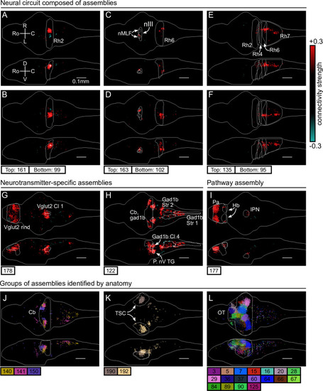
(A–I) Individual example assemblies μ are shown by coloring each neuron $i$ $i$ with its connectivity weight value $w_{i, μ}$ $w_{i, μ}$ (see color bar at the right hand side). The assembly index μ is stated at the bottom of each panel. The orientation and scale are given in panel A (Ro: rostral, C: caudal, R: right, L: left, D: dorsal, V: ventral). Anatomical regions of interest, defined by the ZBrain Atlas (Randlett et al., 2015), are shown in each panel (Rh: rhombomere, nMLF: nucleus of the medial longitudinal fascicle; nIII: oculomotor nucleus nIII, Cl: cluster; Str: stripe, P. nV TG: Posterior cluster of nV trigeminal motorneurons; Pa: pallium; Hb: habenula; IPN: interpeduncular nucleus). (J–L) Groups of example assemblies that lie in the same anatomical region are shown for cerebellum (Cb), torus semicircularis (TSC), and optic tectum (OT). Neurons i were defined to be in an assembly μ when $| w_{i, μ} | > 0.15$ $| w_{i, μ} | > 0.15$ , and colored accordingly. If neurons were in multiple assemblies shown, they were colored according to their strongest-connecting assembly.

Figure 4

HU dynamics are bimodal and activate slower than neurons.

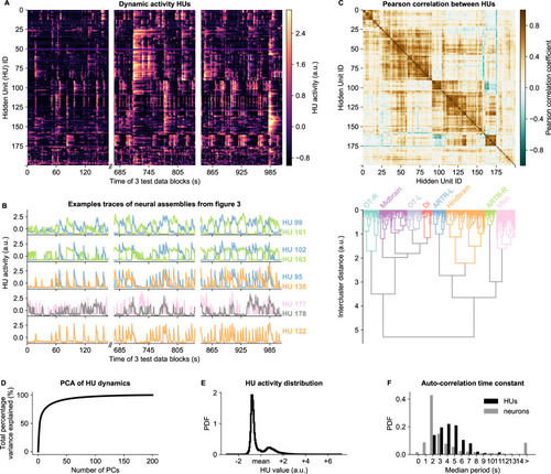
(A) HU dynamics are diverse and are partially shared across HUs. The bimodality transition point of each HU was determined and subtracted individually, such that positive values correspond to HU activation (see Materials and methods - ‘Time constant calculation’6.12). The test data consisted of three blocks, with a discontinuity in time between the first and second block (Materials and methods). (B) Highlighted example traces from panel A. HU indices are denoted on the right of each trace, colored according to their cluster from panel D. The corresponding cellular assemblies of these HU are shown in Figure 3A-I. (C) Top: Pearson correlation matrix of the dynamic activity of panel A. Bottom: Hierarchical clustering of the Pearson correlation matrix. Clusters (as defined by the colors) were annotated manually. This sorting of HUs is maintained throughout the manuscript. OT: Optic Tectum, Di: Diencephalon, ARTR: ARTR-related, Misc.: Miscellaneous, L: Left, R: Right. (D) A Principal Component Analysis (PCA) of the HU dynamics of panel A shows that much of the HU dynamics variance can be captured with a few PCs. The first 3 PCs captured 52%, the first 10 PCs captured 73% and the first 25 PCs captured 85% of the explained variance. (E) The distribution of all HU activity values of panel A shows that HU activity is bimodal and sparsely activated (because the positive peak is smaller than the negative peak). PDF: Probability Density Function. (F) Distribution of the time constants of HUs (black) and neurons (grey). Time constants are defined as the median oscillation period, for both HUs and neurons. An HU oscillation is defined as a consecutive negative and positive activity interval. A neuron oscillation is defined as a consecutive interspike-interval and spike-interval (which can last for multiple time steps, for example see Figure 1A). The time constant distribution of HUs is greater than the neuron distribution (Mann Whitney U test, $P < 10^{- 16}$ $P < 10^{- 16}$ ).

Figure 5

cRBM gives rise to functional connectivity that is strongly correlated across individuals.

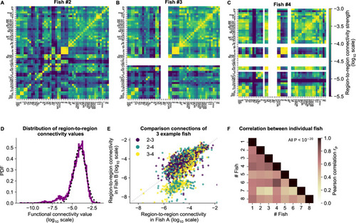
(A) The functional connectivity matrix between anatomical regions of the mapzebrain atlas (Kunst et al., 2019) of example fish #2 is shown. Functional connections between two anatomical regions were determined by the similarity of the HUs to which neurons from both regions connect to (Materials and methods). Mapzebrain atlas regions with less than five imaged neurons were excluded, yielding $N_{MAP} = 50$ $N_{MAP} = 50$ regions in total. See Supplementary file 1 for region name abbreviations. The matrix is shown in log₁₀ scale, because functional connections are distributed approximately log-normal (see panel D). (B) Equivalent figure for example fish #3 (example fish of prior figures). (C) Equivalent figure for example fish #4. Panels A-C share the same log₁₀ color scale (right). (D) Functional connections are distributed approximately log-normal. (Mutual information with a log-normal fit (black dashed line) is 3.83, while the mutual information with a normal fit is 0.13). All connections of all eight fish are shown, in log₁₀ scale (purple). (E) Functional connections of different fish correlate well, exemplified by the three example fish of panels A-C. All non-zero functional connections (x-axis and y-axis) are shown, in log₁₀ scale. Pearson correlation $r_{P}$ $r_{P}$ between pairs: $r_{P} (# 2, # 3) = 0.73$ $r_{P} (# 2, # 3) = 0.73$ , $r_{P} (# 2, # 4) = 0.73$ $r_{P} (# 2, # 4) = 0.73$ , $r_{P} (# 3, # 4) = 0.78$ $r_{P} (# 3, # 4) = 0.78$ . All correlation p values $< 10^{- 20}$ $< 10^{- 20}$ (two-sided t-test). (F) Pearson correlations $r_{P}$ $r_{P}$ of region-to-region functional connections between all pairs of 8 fish. For each pair, regions with less than five neurons in either fish were excluded. All p values $< 10^{- 20}$ $< 10^{- 20}$ (two-sided t-test), and average correlation value is 0.69.

Figure 6

cRBM-inferred functional connectivity reflects structural connectivity.

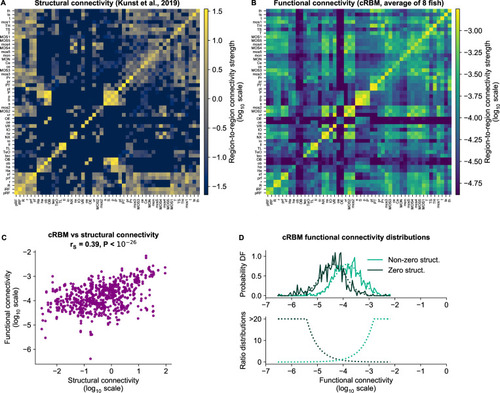
(A) Structural connectivity matrix is shown in log₁₀ scale, updated from Figure 8C of Kunst et al., 2019. Regions that were not imaged in our experiments were excluded (such that $N_{MAP} = 50$ $N_{MAP} = 50$ out of 72 regions remain). Regions (x-axis and y-axis) were sorted according to Kunst et al., 2019. Compared to Figure 8C of Kunst et al., 2019 additional structural data was added and the normalization procedure was updated to include within-region connectivity (see Materials and methods - ‘Extensions of the structural connectivity matrix’). See Supplementary file 1 for region name abbreviations. (B) Average functional connectivity matrix is shown in log₁₀ scale, as determined by averaging the cRBM functional connectivity matrices of all 8 fish (see Materials and methods - ‘Specimen averaging of connectivity matrices’). The same regions (x-axis and y-axis) are shown as in panel A. (C) The average functional and structural connectivity of panels A and B correlate well, with Spearman correlation $r_{S} = 0.39$ $r_{S} = 0.39$ ( $P < 10^{- 20}$ $P < 10^{- 20}$ , two-sided t-test). Each data point corresponds to one region-to-region pair. Data points for which the structural connection was exactly 0 were excluded (see panel D for their analysis). (D) The distribution of average functional connections of region pairs with non-zero structural connections is greater than functional connections corresponding to region pairs without structural connections ( $P < 10^{- 15}$ $P < 10^{- 15}$ , two-sided Kolmogorov-Smirnov test). The bottom panel shows the evidence for inferring either non-zero or zero structural connections, defined as the fraction between the PDFs of the top panel (fitted Gaussian distributions were used for denoising).

Acknowledgments

This image is the copyrighted work of the attributed author or publisher, and ZFIN has permission only to display this image to its users. Additional permissions should be obtained from the applicable author or publisher of the image. Full text @ Elife

van der Plas et al., 2023

ZDB-PUB-230118-3
PMID:36648065

Neural assemblies uncovered by generative modeling explain whole-brain activity statistics and reflect structural connectivity

cRBMs construct Hidden Units by grouping neurons into assemblies.

cRBM is optimized to accurately replicate data statistics.

cRBM assemblies compose functional circuits and anatomical structures.

HU dynamics are bimodal and activate slower than neurons.

cRBM gives rise to functional connectivity that is strongly correlated across individuals.

cRBM-inferred functional connectivity reflects structural connectivity.

van der Plas et al., 2023 ZDB-PUB-230118-3 PMID:36648065

Neural assemblies uncovered by generative modeling explain whole-brain activity statistics and reflect structural connectivity

cRBMs construct Hidden Units by grouping neurons into assemblies.

cRBM is optimized to accurately replicate data statistics.

cRBM assemblies compose functional circuits and anatomical structures.

HU dynamics are bimodal and activate slower than neurons.

cRBM gives rise to functional connectivity that is strongly correlated across individuals.

cRBM-inferred functional connectivity reflects structural connectivity.

van der Plas et al., 2023

ZDB-PUB-230118-3
PMID:36648065