
- Title
-
Optic flow in the natural habitats of zebrafish supports spatial biases in visual self-motion estimation
- Authors
- Alexander, E., Cai, L.T., Fuchs, S., Hladnik, T.C., Zhang, Y., Subramanian, V., Guilbeault, N.C., Vijayakumar, C., Arunachalam, M., Juntti, S.A., Thiele, T.R., Arrenberg, A.B., Cooper, E.A.
- Source
- Full text @ Curr. Biol.
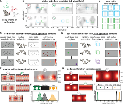
Spatial biases in optic flow sampling for self-motion estimation improve performance
(A) We consider the optic flow generated by 6 components/directions of self-motion including translation and rotation, illustrated for a moth. (B) Idealized optic flow templates for recovering each component of self-motion in a spherical environment are shown across the full visual field. (C) For the blue and green regions highlighted in (B), we show the local flow templates for a 10° square region under a tangent projection. A small field of view can lead to a high degree of similarity between translation and rotation template patches (e.g., VX and ωY look very similar locally at these two positions but are more distinguishable with the full field of view). Arrowheads for the templates located at foci of expansion/contraction have been scaled up for visibility. (D) To model self-motion estimation from sparse, noisy optic flow across the full visual field, we randomly sampled 60 visual field locations (of 180 predetermined possible locations) and calculated the median absolute self-motion estimation error for each component. Once a sample set was chosen, self-motion components were drawn uniformly at random from −1 to 1 (m/s for translation and rad/s for rotation), and additive Gaussian noise of standard deviation of 0.25 (relative to a maximal per-component flow magnitude of 1) was applied to the resulting flow vectors. The environment was modeled as a 1-m radius sphere. Each row illustrates one iteration of the model: we ran 10,000 iterations with different sample locations each time, and each iteration included 10,000 random self-motions for computing the median absolute error. Color bars indicate the median self-motion estimation error associated with each sample set. We then computed the overall median absolute error (median of medians) associated with each visual field sample location across all iterations. (E) Heatmaps show the overall median absolute errors associated with each sample location for each self-motion component, with VZ plotted larger for visibility. The heatmap ranges for the other components are: VX (2.59,2.61), VY (2.94,2.99), ωX (1.48,1.50), ωY (1.68,1.71), and ωZ (1.48,1.50). (F) Histograms illustrate the median VZ estimation error when 50% of the sample locations were used. These 50% could be spread evenly across the visual field (black), concentrated away from the VZ foci of expansion/contraction (green) or concentrated at these foci (orange). The anti-focus spatial bias leads to better estimates. We fitted each distribution with a Gaussian and computed the effect size (the difference between the means normalized by the pooled standard deviations) between the full field and biased samples as follows: anti-foci versus full field = −3.6; foci versus full field = 5.0. (G) To model self-motion estimation from sparse, noisy optic flow using contiguous local visual field regions similar to receptive fields, we repeated this analysis on small, spatially contiguous regions. Each contiguous region subtended a 10° square and contained up to 100 contiguous optic flow samples, each of which had a 67% chance of being deleted after noise was added, with self-motion and additive noise sampled as before. (H) Heat maps of the resulting median absolute errors. The heatmap ranges for the non-VZ translation components are the same as the VZ plot, and for the rotation components, they range from 20 to 350 deg/s. (I) Histograms illustrate the median VZ estimation error (log-spaced) for the best local region (located at the VZ focus), the worst local region (located at the antifocus), and a region mid-way between those two. Effect sizes are as follows: focus versus mid-way = −64.8; anti-focus versus mid-way = 9.2. |
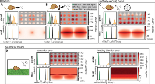
Animal behavior and environment shape spatial biases
(A) An animal only moving forward removes the ambiguity in local flow templates so that both global and local errors indicate an away-from-foci advantage. Histograms on the left indicate the distribution of median absolute self-motion estimation errors for the best 50%, worst 50%, and full field global samples at matched resolution, and the best, worst, and median local regions over 1,000 simulations of 1,000 self-motion trajectories. Heatmaps indicating median errors are plotted in the same format as Figure 1. All model parameters are the same as Figure 1, except self-motion components other than VZ were all set to zero and a 1 DOF estimation applied. For the local optic flow, both the best and median regions are associated with very low error, resulting in a high degree of histogram overlap. (B) An animal translating and rotating in a plane sees higher errors and expanded regions of ambiguity. All model parameters are the same as Figure 1, except self-motion components other than VZ, VX, and ωY were all set to zero and a 3 DOF estimation applied. (C) When noise varies linearly from none at 90° elevation to a maximum at −90° elevation, low error regions are shifted upward. All model parameters are otherwise the same as (B), and maximum noise had a standard deviation of 0.25 (relative to a maximal per-component flow magnitude of 1). (D) When the environment is a floor plane rather than a sphere, VZ error explodes at and above the equator. Heading estimates remove the depth ambiguity in translation component magnitude by comparing VX and VZ estimates, eliminating azimuth dependence for a pure lower field bias. All model parameters are the same as (B) except for the scene geometry, which is modeled as a flat floor 1m below and an infinitely far away wall in the upper visual field. Note that histograms and heatmaps for local errors in this figure are all on a log scale to account for the larger variability associated with different environmental settings. |
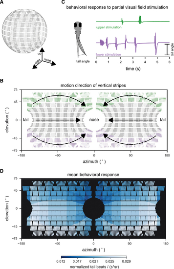
Larval zebrafish optomotor swimming is driven by the lateral lower visual field
(A) Layout of individual LEDs in our spherical visual stimulation arena. The visual stimulus consisted of a pattern of vertical bars meant to simulate the fish swimming through a pipe with transverse stripes. Fish were placed in the center of the spherical arena, thus allowing for stimulation of an extended range of elevations (almost 140° × 360° of its visual field). (B) During individual trials, stripes in different regions of the visual field were moving (example areas marked green or purple), whereas the rest remained static. Stimulus motion was from back to front, providing the percept of backward drift to the fish. (C) Tail bend angles were measured for each recorded video frame to calculate behavioral responses to different stimulus locations. Fish generally responded more strongly to motion in the lower (purple trial), than in the upper (green trial) visual field. (D) Heatmap color indicates the strength of the OMR to motion stimuli in different parts of the visual field. OMR drive was strongest for motion in the lateral lower visual field. To quantify the behavioral response, the number of tail beats per unit time was averaged over repeated trials for each fish, normalized by the fish’s maximum response to any of the stimuli, and scaled by the inverse of the area (in steradians) that was active (i.e., moving) for each stimulus to account for effects of stimulation area size on response strength. Responses were then combined into a single average across fish (n = 8 fish). Motion stimuli covered 19 different combinations of positions and steradian sizes in visual space. See also Figure S1. |
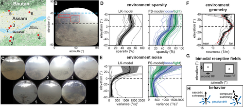
A model for natural optic flow statistics during zebrafish self-motion
(A) Seven sites in the native range of the zebrafish were sampled, see Table S1 for details. Image from Google Maps.55 (B) An equirectangular projection of a sample frame shows elevation-dependent sources of signal and noise. (C) Frames from each site summarize visual variation across the native range. (D) Optic flow sparsity at individual sites (thin lines) and averaged across the dataset (thick lines, ±SEM in filled region) show high sparsity near and above the equator. This pattern holds across motion measurement algorithms (black, blue, and green). (E) Errors in optic flow, attributed to natural motion within the environment, show higher variance in the upper visual field. (F) The geometry estimated from optic flow vector magnitudes roughly matches a floor+ceiling model (dashed red) below the water line (~40°). Individual sites, SEM, and mean are plotted in the same manner as in (D) and (E). (G) Receptive field structure is modeled in spatially separate bimodal pairs. Base RFs were placed in a predetermined grid of locations and paired with a range of possible second RFs. (H) Two swimming behaviors are considered: saccadic swimming, where forward motion is added to lateral drifting (VZ ~ U[0,1] m/s + (VX,VZ) ~ U[−.5, −.5] m/s) and compound swimming, which additionally includes rotation (ωY ~ U[−1,1] rad/s). For more details, see Figures S1–S3 and S7, Video S1, and Tables S1–S4. |
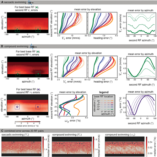
The visual ecology of the larval zebrafish generates lower translation estimation errors in the lateral lower field
Data were simulated using naturalistic models of signal sparsity and noise, environment geometry, RF size and structure, and swimming behaviors. For each possible base RF location (see legend in B), median absolute errors were computed for 10,000 iterations across all second RF locations. (A) Left: for saccadic swimming, the lowest error occurred when the base and second RF were located at an elevation of −60° and had azimuths of 90° and −90°, respectively. The plot shows a heatmap of the median absolute VZ error over across all second RF locations for the best base RF, and the single best base/second pair is indicated with an x and o. middle: for VZ and heading error, median absolute errors are averaged across azimuths to isolate elevation trends for each base RF location (colors indicate base RF elevation, line thicknesses indicate base RF azimuth). Both metrics show that translation is best recovered by RF pairs in the lower visual field. Right: When averaging across elevation for azimuth trends, the lower field base RFs tend to be best matched with a second RF at ±90° azimuth. For clarity, we only plot the results for the best base elevation (−60°). (B) For compound swimming behavior, local translation errors (top left) show more extreme penalties for same-side sampling due to ambiguity with rotation. Elevation trends (top middle) are largely unaffected, other than an increase in average error, but azimuth trends (top right) show a strong advantage to sampling the lateral region on the other side of the body. The azimuth and elevation of the best individual pair are the same as for saccadic swimming. For rotation estimation (bottom), the lower field advantage is less strong, and the best performing bimodal RF (bottom left) appears at −20° elevation. Elevation trends (bottom middle) show strong performance throughout the lower field, whereas azimuth trends show no clear advantage to lateral regions, instead suggesting an azimuth separation of 180° minimizes error (bottom right). Full error maps can be seen in Figures S4 and S5, with a comparison across flow calculation methods shown in Figure S6. (C) To characterize the performance across the visual field, we followed a similar method to the global method described in the previous section. Instead of a location sample corresponding to a single flow vector, we sampled sets of 20 RF pairs, with one centered at the sample location and the other 180° away in azimuth at the same elevation. The median absolute error over 1,000 estimates is shown for each of the motion directions from (A) and (B). Again, we see better performance in the extreme lower field for translation estimation (left, middle) and in the mid-lower field for rotation (right). See also Figures S4–S6. |
Ignoring the upper field improves motion estimates from optic flow measured in the native habitat of the zebrafish
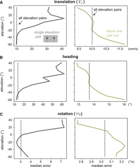
We demonstrate the value of spatial biases by showing an advantage to excluding elevations from self-motion estimation across our dataset of natural optic flows. For velocity distribution and dataset size, see Table S2. (A–C) We consider forward translation (A), heading (B), and rotation (C) errors for single RFs pairs, comparing with a baseline of using all elevations (dotted vertical line). When using a single elevation (first column), the best regions predicted by our simulations are equal to or outperform the baseline. When all but one elevations are used (second column), removing lower field samples damages performance while removing upper field samples improves it. |
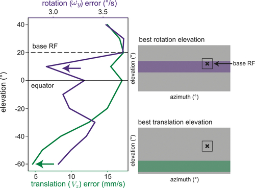
Spatially varying resolution of the front end of the sensory system can shift rotation bias
Beginning with the compound swimming setting in Figure 5, we modified our sparsity model to increase sample probability by a factor of 4 in the upper visual field, as a proxy for higher retinal resolution. In this setting, a base receptive field located at 20° elevation (black dashed line) and 90° azimuth is better paired with another upper field RF for rotation (purple arrow) while still benefiting from a lower field partner for translation (green arrow). Compare with Figure 5D in which both types of motion estimation show lower error in the lower field. Spatial variations in anatomical resolution may be responsible for a slight upper field bias observed in rotation responses in the larval zebrafish. |