
|
Fig. 4
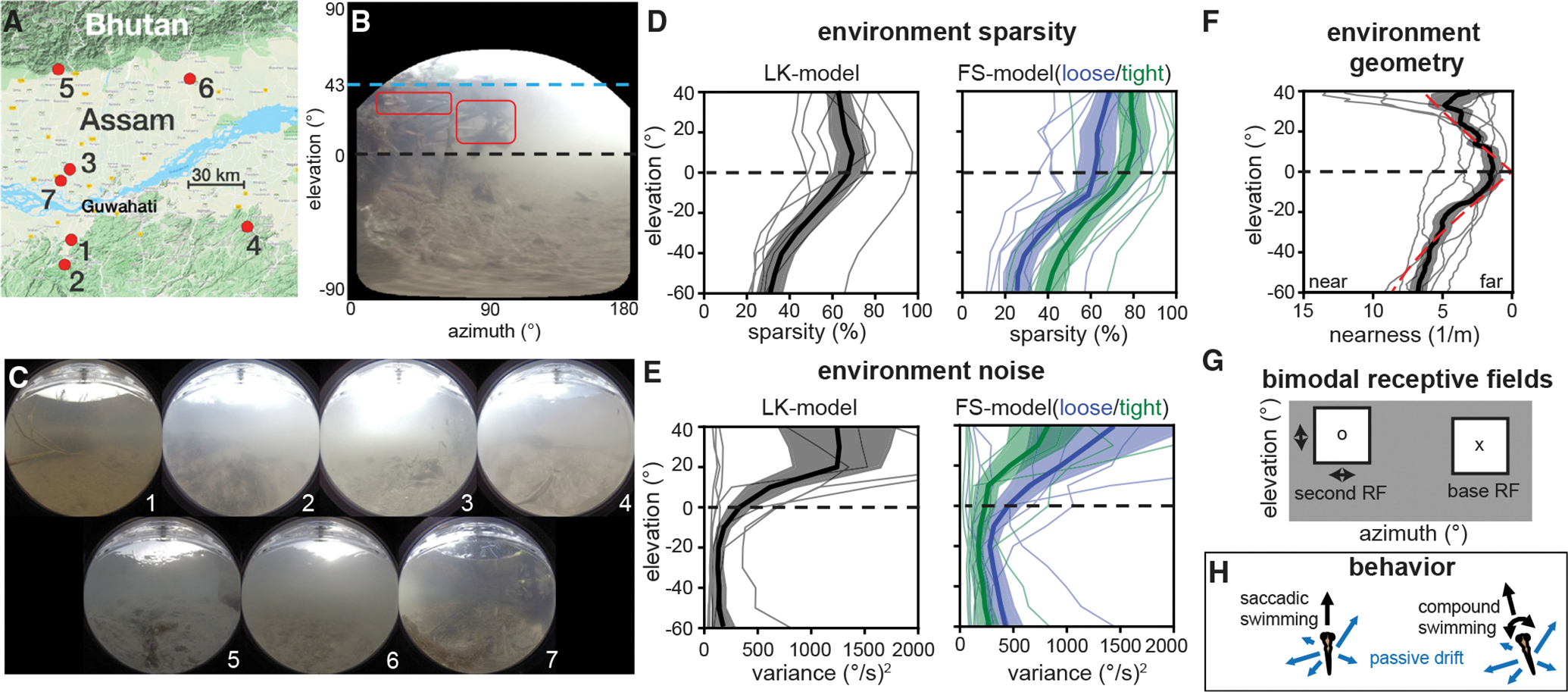
(A) Seven sites in the native range of the zebrafish were sampled, see Table S1 for details. Image from Google Maps.55
(B) An equirectangular projection of a sample frame shows elevation-dependent sources of signal and noise.
(C) Frames from each site summarize visual variation across the native range.
(D) Optic flow sparsity at individual sites (thin lines) and averaged across the dataset (thick lines, ±SEM in filled region) show high sparsity near and above the equator. This pattern holds across motion measurement algorithms (black, blue, and green).
(E) Errors in optic flow, attributed to natural motion within the environment, show higher variance in the upper visual field.
(F) The geometry estimated from optic flow vector magnitudes roughly matches a floor+ceiling model (dashed red) below the water line (~40°). Individual sites, SEM, and mean are plotted in the same manner as in (D) and (E).
(G) Receptive field structure is modeled in spatially separate bimodal pairs. Base RFs were placed in a predetermined grid of locations and paired with a range of possible second RFs.
(H) Two swimming behaviors are considered: saccadic swimming, where forward motion is added to lateral drifting (VZ ~ U[0,1] m/s + (VX,VZ) ~ U[−.5, −.5] m/s) and compound swimming, which additionally includes rotation (ωY ~ U[−1,1] rad/s). For more details, see Figures S1–S3 and S7, Video S1, and Tables S1–S4.