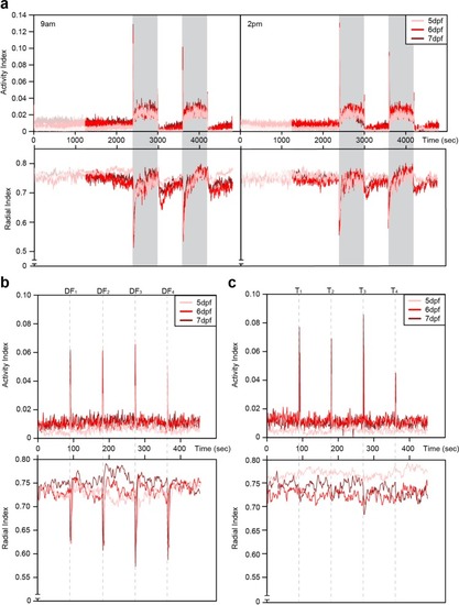
Time series plots from behavior experiments. (a) Average activity index (top) and radial index (bottom) per second of 132 zebrafish larvae over the study period under light or dark period at either 9 am (left) or 2 pm (right) for 5, 6 or 7 dpf. Initial 20 minutes acclimation period (faded period), followed by 20 minutes of “spontaneous” swimming, then swimming under darkness (2 × 10 min, referred to as “dark intervals”, shaded period) and swimming in light after periods of darkness (2 × 10 min, referred to as “light intervals”). For the startle triggers of (b) dark flashes (DF) and (c) tapping (T), average activity for 9 am measurements are shown. The dashed grey lines indicate occurrence of the stimuli.

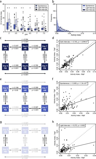
Behavioral intra-individual variability in a population of 132 larvae for the activity index. (a) Boxplot of the coefficient of variation of activity index for each individual larva (n = 132) over the different days (days post fertilization; dpf) under the different conditions studied. (b) Frequency distribution of the activity index in spontaneous, light and dark intervals depicting the differential activity profiles under these conditions. Schematics represent correlations of activity between different days and times of day for each of the conditions of study, (c) dark intervals, (e) spontaneous and (g) light intervals. Correlation plots between activity of larvae on day 6 vs 7 for (d) dark intervals, (f) spontaneous and (h) light intervals. Statistics on the plots represent the Pearson’s correlation coefficient and respective p value, with a linear regression line fitted for visual aid on the scatter plots (black solid line) and unity line (grey dashed line).

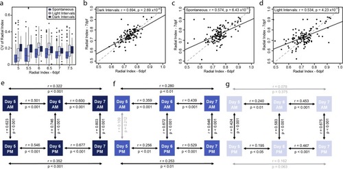
Behavioral intra-individual variability in a population of 132 larvae for the radial index. (a) Boxplot of the coefficient of variation of radial index for each individual larva (n = 132) over the different days (days post fertilization; dpf) under the different conditions studied. Correlation plots between the radial index of larvae on day 6 vs 7 for (b) dark intervals, (c) spontaneous and (d) light intervals. Schematics represent correlations of the radial index between different days and times of day for each of the conditions of study, (e) dark intervals, (f) spontaneous and (g) light intervals. Statistics on the plots represent the Pearson’s correlation coefficient and respective p value, with a linear regression line fitted for visual aid on the scatter plots (black solid line) and unity line (grey dashed line).

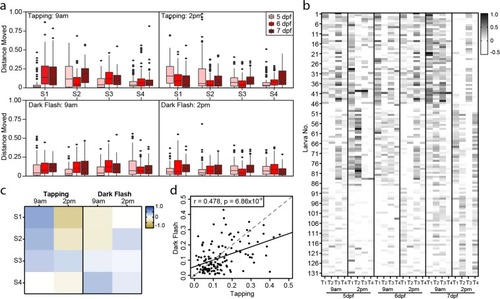
Individual responses to startle stimulus. (a) Boxplots of the average distance moved of the 132 larvae at each of the four stimuli (S1–S4) (tap or dark flash) at either 9 am or 2 pm. The different color boxes represent the three different days measured on 5, 6 and 7 days post fertilization (dpf). (b) Heat map representing the change in distance moved with respect to the baseline of each individual larva for all time points and days measured in response to each of the tapping stimulus (T1–T4). White represents no response to the stimulus, with the grey scale darkening in a linear scale depending on the strength of the response. (c) Heat map of the r values from the correlations of distance moved of individual larvae between 6 and 7 dpf, for each of the four startle stimuli at either 9 am or 2 pm for tapping and dark flashes. Blue represents a positive correlation, with yellow representing a negative correlation. (d) Correlation plot between the individual fish response to the first dark flash and the first tap at 6 dpf. Each point on the graph represents an individual larva (n = 132) and the correlation coefficient was calculated using Pearson’s correlation, with a linear regression line fitted for visual aid (black solid line) and unity line (grey dashed line).

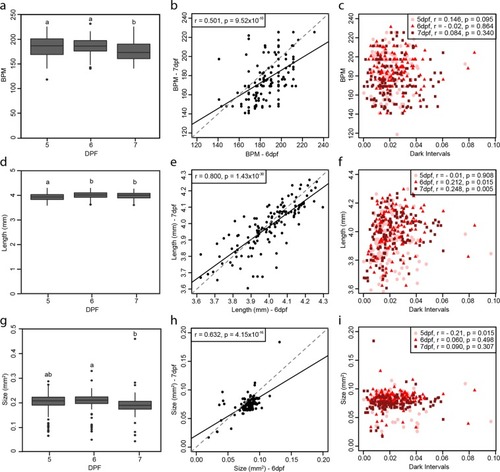
Physiology and morphometric parameter comparisons. Boxplots representing the average measure of all 132 larvae of (a) heart rate (beats per minute; BPM) (one-way ANOVA: F_{(2, 393)} = 9.73, p < 0.001 followed by Tukey HSD multiple comparison: p _(5dpf-6dpf) = 0.92, p _(5dpf-7dpf) < 0.01, p _(6dpf-7dpf) < 0.001), (d) body length (mm) (one-way ANOVA: F_{(2, 393)} = 54.328, p < 0.001 followed by Tukey HSD multiple comparison: p _(5dpf-6dpf) < 0.001, p _(5dpf-7dpf) < 0.001, p _(6dpf-7dpf) = 0.99) and (g) size of swim bladder (mm²) (one-way ANOVA: F_{(2, 393)} = 5.31, p < 0.01 followed by Tukey HSD multiple comparison: p _(5dpf-6dpf) = 0.255, p _(5dpf-7dpf) = 0.215, p _(6dpf-7dpf) < 0.01), over the three days of experiments (5, 6 and 7 days post fertilization, dpf) with significant difference represented by different letters on each graph. Correlation plots between 6 and 7 dpf for (b) heart rate, (e) body length and (h) size of swim bladder, with each point representing a single larva. Comparison of the individuals’ (c) heart rate, (f) body length and (i) size of swim bladder to their respective average activity during dark intervals, with each day plotted on each plot (5 dpf: circle, 6 dpf; triangle and 7 dpf; square). Statistics on the plots represent the Pearson’s correlation coefficient and respective p value, with a linear regression line fitted for visual aid on the scatter plots (black solid line) and unity line (grey dashed line).