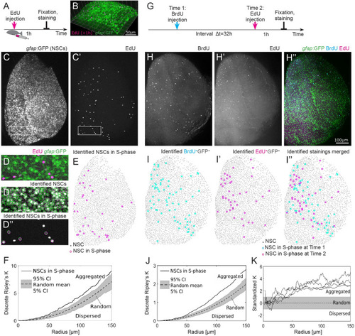
(A) Experimental setup: EdU is injected intraperitoneally 1 h prior to humanely killing the fish and fixation of the brain. (B) Part of the telencephalic hemisphere as a 3D reconstruction. The gfap:GFP transgene highlights cell bodies of NSCs, which are arranged on a 2D layer on the telencephalon surface, while their radial processes project deep in the parenchyme. (C, C’) gfap:GFP in the whole hemisphere shown as a maximum intensity z-stack projection, anterior to the top, lateral to the right, and medial to the left. Boxed areas are shown as higher magnifications in (D–D”). (C’) EdU coupled to Azyde-Alexa 647 highlights cells in S-phase and reveals their spatial distribution. (D) Merged GFP and EdU channel to identify specifically the NSCs in S-phase. (D’) Automatically identified NSCs surrounded by green circles. (D”) EdU+ cells were subdivided into EdU+gfap:GFP− and EdU+gfap:GFP+, the latter representing NSCs in S-phase. (E) The 33 NSCs in S-phase (pink circles) exhibit a nonrandom spatial pattern on top of all 2678 NSCs (gray dots). (F) Discrete Ripley’s K quantification of the pattern shown in (E) reveals that NSCs in S-phase (solid line) are aggregated, i.e., closer to each other than expected from random (dotted line with 90% CI in gray) and dispersed patterns. (G) Cells in S-phase are labeled with BrdU and EdU with an interval of 32 h. Fish are humanely killed 1 h after the EdU injection, and the brains are imaged after fixation and staining. (H–H”) Example of 1 telencephalic hemisphere, oriented as in (C), as a maximum intensity z-stack projection, in 3 different channels: BrdU (H), EdU (H’), and gfap:GFP transgene highlighting NSC bodies merged with the EdU and BrdU staining (H”). Scale bar: 100 μm. (I–I”) Identified NSCs in S-phase at 2 different time points exhibit aggregated spatiotemporal patterns. (J) Discrete Ripley’s K reveals more EdU+ NSCs around BrdU+ NSCs as expected from a random process. (K) We find spatiotemporally aggregated patterns with radii above 50 μm in all 4 hemispheres where S-phases have been labeled with a labeling interval of 32 h. BrdU, 5-bromo-2′-deoxyuridine; CI, confidence interval; EdU, 5-Ethynyl-2′-deoxyuridine; GFP, green fluorescent protein; NSC, neural stem cell.

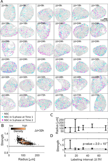
(A) Our dataset comprises 36 hemispheres with labeling intervals from Δt = 9 h to 72 h. (B) Posterior sampling identifies the most likely interaction strength of 1.15 and most likely interaction radius of 98 μm for 4 Δt = 32 h hemispheres. Whiskers (gray) cover the 95% CIs for strength and radius. Sampling point density is visualized from copper (high) to black (low). (C) Applied to all 36 hemispheres posterior sampling reveals an interaction radius around 100 μm. (D) The interaction strength is significantly above 1 for all labeling intervals Δt (p-value = 0.0002 for constant fit to most likely values) thus inducing aggregated patterns. CI, confidence interval; NSC, neural stem cell.

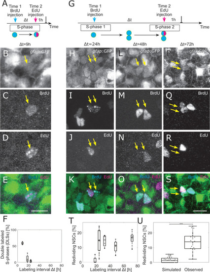
(A) The 2 injections label the same cells in S-phase for small-labeling intervals, leading to NSCs that are both EdU and BrdU positive, denoted as double-labeled S-phase (DLS). (B–E) Example DLS (yellow arrow) for a labeling interval Δt = 9 h. (F) The DLS proportion is high for Δt = 9 h and decreases rapidly with increasing Δt. Each dot represents the value for 1 brain hemisphere. (G) After a division, 1 of the daughter cells already labeled by the Time 1 label can enter in a new S-phase and incorporate a second label. This cell thereby redivides. (H–S) Three examples of redividing NSCs with labeling intervals of 24 h (H–K), 48 h (L–O), and 72 h (P–S). Scale bar: 10 μm. (T) The proportions of redividing NSCs within the dividing NSCs at Time 1 remain high from Δt = 24 h to Δt = 72 h labeling intervals. Each dot represents 1 brain hemisphere. (U) Only 1.9±1.7% of randomly drawn divisions (same amount as observed per hemisphere) from all NSCs would be redrawn at random, while 14±8% of observed NSCs in S-phase reenter S-phase (p = 9.4 ×·10⁻¹⁰, 2-sample Kolmogorov–Smirnov test). Box plots range from the 25th to the 75th percentile, and the central mark indicates the median and whiskers include points that are not more than 1.5 times the interquartile range away from the top or bottom of the box. BrdU, 5-bromo-2′-deoxyuridine; DLS, double-labeled S-phase; EdU, 5-Ethynyl-2′-deoxyuridine; GFP, green fluorescent protein; NSC, neural stem cell.

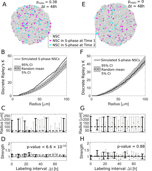
(A) We use an agent-based model to simulate NSC divisions with a redivision probability of p_rediv = 0.38 and perform virtual measurements with labeling intervals Δt between 9 h and 72 h (here shown for Δt = 48 h). (B) The simulated NSCs in S-phase in (A) exhibit an aggregated spatiotemporal pattern according to the discrete Ripley’s K curve (solid line) which is above the 90% CI of randomly sampled patterns (gray area), similar to experimentally observed patterns. (C) The fitted radii for simulations with redividing NSCs for different labeling intervals Δt are variable with a maximum likelihood value of 50 μm. Labeling intervals that are also available from experimental data (see Fig 2C) are shown in black, all others in gray. (D) The respective fitted strengths values are above 1 indicating aggregated patterns. Fitting a constant model to the most likely values with the same Δt as experimentally observed (black bars) reveals a significant shift (p-value = 6.6 × 10⁻¹⁰) from a strength of 1. Labeling intervals that are also available from experimental data (see Fig 2D) are shown in black, all others in gray. (E) Simulated NSC divisions and virtual measurements with a redivision probability p_rediv = 0 at 2 labelings Δt = 48 h apart. (F) Without redivisions, the simulated S-phase NSCs are within the boundaries of random patterns. (G) The fitted radii are highly variable with maximum likely values from 50 to 150 μm. Labeling intervals that are also available from experimental data (see Fig 2C) are shown in black, all others in gray. (H) In contrast to the simulations with redivisions, we now find no indication for aggregated patterns for all labeling intervals (p-value = 0.88 for a constant model with nonzero shift from a strength of 1). Labeling intervals that are also available from experimental data (see Fig 2D) are shown in black, all others in gray. CI, confidence interval; NSC, neural stem cell.