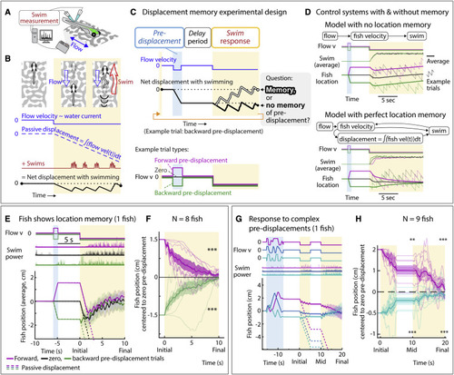
Larval zebrafish track their spatial location and correct for unintended displacements

(A) Experimental setup: larval zebrafish fictively swimming in a virtual reality environment.

(B) Fish swim in response to virtual flow so that their net displacement is smaller than the passive displacement. Dashed lines show passive displacements here and in later figures.

(C) Experimental design: fish undergo one of various forced trajectories (blue pre-displacement period). After a delay period (white), they can correct for the pre-displacement by swimming the correct amount against a virtual flow in “closed loop” (yellow swim period).

(D) Simulated fish behavior showing two classes of outcomes. If average trajectories during forward versus backward pre-displacements converge during the swim period, it implies fish have memory of self-location.

(E) Example fish behavior in pre-displacement experiment. Average trajectories for the three trial types approximately converge at ∼5 s, showing that this fish has memory of pre-displacement. (Shaded regions, SEM in all panels.)

(F) Trajectories (8 fish) normalized and centered to zero pre-displacement trajectory converge at ∼10 s, indicating accurate memory of previous location shift. (One-sample t test for final positions, ^∗∗∗p < 0.001, p = 7.3e−8 for backward pre-displacement, specified mean = −1; p = 6.3e−7 for forward pre-displacement, specified mean = 1.)

(G) Assay to test integration during stochastic pre-displacements and to examine corrections made over two swim periods separated by a delay. This example fish successfully corrects for stochastic pre-displacements; correction continues across two swim periods.

(H) Population data showing accurate correction distributed over both swim periods, i.e., 1D path integration of complex trajectories. (One-sample t test, ^∗∗p < 0.01, p = 0.0023 for forward pre-displacements at mid time point, ^∗∗∗p < 0.001, p = 2.5e−5 for backward pre-displacements at mid time point. p = 2.1e−7 for forward pre-displacement at final time point, p = 5.8e−8 for backward pre-displacement at final time point. Data shown centered to average of trajectories that integrate to zero.).

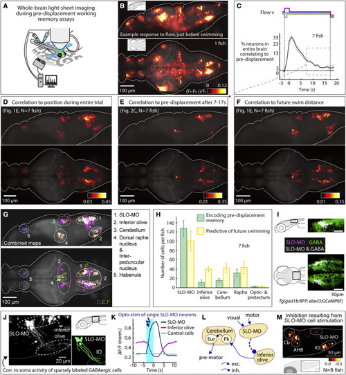
Figure 2. Whole-brain activity maps reveal neural populations encoding self-location

(A) Virtual reality system for paralyzed zebrafish and light-sheet microscope for imaging whole-brain cellular activity.

(B) Example brain-wide activity following forward visual motion, just before swim initiation in Tg(elavl3:GCaMP6f) fish (Figure S5A for earlier and later time points). Shown is the difference between imaging frames F _t-1 and F_t normalized by baseline fluorescence, where F _t+1 are frames containing the first swim bouts occurring after swim period onset.

(C) Fraction of neurons across the brain with significant correlation to pre-displacement direction as a function of elapsed time. At 17 s after the pre-displacement, a fraction of neurons still encodes pre-displacement direction (shaded regions: SEM; arrow refers to time period used for analysis in (E); backward pre-displacement is shorter than forward to limit swimming during pre-displacement).

(D) Whole-brain map of neurons encoding self-location during pre-displacement, delay, and swim periods. Cells with p < 0.005 for Spearman correlation in at least 80% of time points are shown (STAR Methods). Color bar represents averaged Spearman correlation coefficient to location.

(E) Map of neurons encoding self-location during long delay period (C). Cells with p < 0.005 for Spearman correlation to self-location at every time point between 7 and 17 s are shown. Color bar represents averaged Spearman correlation coefficient of all time points.

(F) Map of neurons whose activity at swim period onset (before first swim bout) predicts total distance swum in swim period. Cells with p < 0.005 for Spearman correlation at first two time points in the swim period are shown. Color bar represents averaged Spearman correlation coefficient.

(G) Combined maps of (D)–(F) listing brain areas containing neurons potentially involved in self-localization.

(H) Numbers of identified neurons (cell segments) per fish per area encoding memory of location during pre-displacement and delay periods, and numbers of neurons predicting future distance swum in the swim period. (Error bars, SEM.)

(I) Dorsal hindbrain map of SLO-MO neurons and GABAergic neurons in Tg(elavl3:GCaMP6f; gad1b:RFP) showing strong overlap between SLO-MO and GABAergic populations (white).

(J) Hybrid functional and anatomical tracing of SLO-MO neurites through sparse expression in Tg(gad1b:Gal4; UAS:GCaMP6f) using fluorescence correlation to SLO-MO cell body activity to help distinguish neurites in sparse gad1b line, showing innervation of IO (STAR Methods).

(K) Optogenetic activation SLO-MO (single neurons of any functional type; STAR Methods) using CoChR⁵⁹ in Tg(gad1b:Gal4; UAS:CoChR; elavl3:jRGECO1b) (see Figures S7K and S7L) shows IO neurons are inhibited during SLO-MO activation, indicating functional connection consistent with GABAergic inhibition.

(L) Local circuit diagram of hypothesized SLO-MO inhibition of IO (dashed line) and known circuitry from IO to Cb cell types (Pk, Purkinje cells; Eur, eurydendroid cells, homologous to deep cerebellar nuclei).

(M) Hindbrain functional map of decreases in cell activity (color bar, relative decrease ΔF/F) during SLO-MO activation (one neuron at a time) showing activity reduction in IO, cerebellum, anterior hindbrain (AHB), and non-stimulated SLO-MO cells.

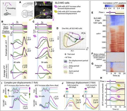
SLO-MO neuronal activity encodes self-location

(A) Location of neurons with increasing activity following backward (yellow) versus forward (magenta) pre-displacement in example fish.

(B) Examples (top) and average (bottom, with ΔF/F during no-displacement trials subtracted) of neurons with increasing activity following backward pre-displacement. (Shaded regions: SEM in all panels; here, 2 s forward or 1 s backward pre-displacements.)

(C) Examples (top) and averages (bottom) of neurons with increasing activity following forward pre-displacement.

(D) Principal-component analysis embedding of SLO-MO population activity. Trajectories remain separated throughout delay period, gradually converge and return toward the starting point during swim period.

(E) SLO-MO neuron activity across 9 fish (1,347 cell segments) sorted by Spearman correlation, showing consistent correlation to self-location across trial types.

(F and G) For comparison, lack of correlation to self-location for cells with activity correlating to swim vigor, and for cells in pretectum that show visual encoding.

(H) Averages of ΔF/F (centered to zero pre-displacement, normalized in each fish) of positive- and negative-correlating neurons from (E).

(I) Encoding of self-location by SLO-MO neurons during complex trajectories (example fish).

(J) Encoding of sideways changes in self-location in SLO-MO neurons (example fish).

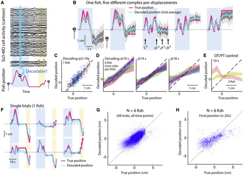
Decoding self-location from SLO-MO neuronal activity

(A) Schematic of self-location decoding from SLO-MO population activity (cartoon data).

(B) Decoding averages of complex location trajectories in pre-displacement and delay periods of stochastic displacement assay (dark gray: standard error [SEM], light gray: standard deviation [SD]). (Fish icons enlarged, not to scale.)

(C) Decoding performance throughout pre-displacement period of example fish.

(D) Decoding performance at start, middle, and end of delay period across N = 6 fish, showing gradually declining performance as SLO-MO memory decays over many seconds (colors: SEM for each fish).

(E) Decoder trained on midbrain visual neurons performs poorly.

(F) Example decoding of single trials, including first swim period.

(G) Decoding self-location during entire trial across N = 7 fish, r = 0.54, p < 0.01.

(H) Performance of decoding self-location at end of swim period (at t = 20 s), r = 0.68, p < 0.01.

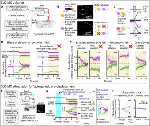
SLO-MO is necessary for location memory and changes future locomotion

(A) Two-photon laser ablation of selected functionally identified SLO-MO neurons in Tg(elavl3:GCaMP6f) fish.

(B) Ablating either population (example shown here: ablation of backward pre-displacement tuned cells) abolishes pre-displacement memory capacity of the entire population but leaves short-timescale sensory responses intact (C), suggesting integration through local connectivity within SLO-MO.

(C) Following ablation of one functional population (here, forward displacement tuned neurons), SLO-MO responses of the remaining population (here, backward-tuned neurons) remain visually responsive but lose their persistence. (Shaded regions: SEM in all panels.)

(D) Ablating neurons tuned positively to forward pre-displacement abolishes positional homeostasis in an example fish.

(E) Population data showing consistent abolishment of positional homeostasis across N = 6 fish after ablation of either the forward or the backward pre-displacement encoding population, but not for nearby control neurons. (One-sample t test, ^∗∗∗p < 0.001, p < 2.5e−5 for all pre-ablation, ^∗∗p < 0.01, p = 3.8e−3 for backward pre-displacements after control ablation, p = 6.4e−2 for forward pre-displacements after control ablation, n.s. p > 0.05. Error bars: SEM in all panels.).

(F) Stimulation setup for activating functionally identified SLO-MO populations using optogenetics in Tg(gad1b:Gal4; UAS:CoChR; elavl3:jRGECO1b) fish.

(G) Optogenetic activation of backward pre-displacement encoding neurons (green) causes increased swimming 5–10 s later, and activation of forward pre-displacement encoding neurons (magenta) causes decreased swimming. Control cells that do not encode location do not affect swimming. Inset: manually shifted trajectories to illustrate the similarity to behavior with visual pre-displacements.

(H) Population data showing consistent increases or decreases in swim distance following stimulation of neurons encoding backward or forward pre-displacements. (15 fish, one-sample t test, ^∗∗∗p < 0.001, p = 4.9e−4 for stimulation of backward-tuned SLO-MO cells, p = 2.1e−6 for stimulation of forward-tuned SLO-MO cells, n.s. p > 0.05, p = 0.15 for stimulation of control cells.).

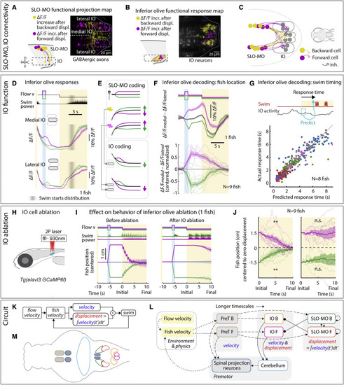
IO is functionally downstream of SLO-MO and necessary for positional homeostasis

(A) Imaging projections from SLO-MO in IO area in Tg(gad1b:Gal4; UAS:GCaMP6f; elavl3:H2B-jRGECO1b). The gad1b channel shows anatomical segregation of projections of SLO-MO neurons that encode forward pre-displacements (projections to medial IO) versus backward pre-displacements (projections to lateral IO). Magenta (yellow) stands for forward-pre-displacement-positive (backward-pre-displacement-positive) SLO-MO cells.

(B) Imaging IO neurons (same fish as in A; pan-neuronal channel shown) showing segregation of neurons responding positively to forward pre-displacements (medial IO) versus backward pre-displacements (lateral IO)—the reciprocal of (A), consistent with inhibition of IO by SLO-MO axons. Magenta (yellow) stands for forward displacements (backward displacements) of fish in VR.

(C) Hypothesized connectivity between SLO-MO and IO based on (A) and (B).

(D) Time courses of IO responses to location changes. Medial IO is persistently suppressed relative to no pre-displacement following backward pre-displacements. Lateral IO is persistently suppressed relative to no pre-displacement following forward pre-displacements. The initial high ΔF/F levels are carried over from the end of the previous swim period (example fish, population data shown in Figures S7N and S7O).

(E) Schematic of location coding in IO versus SLO-MO and connectivity.

(F) Fish location can be decoded from instantaneous IO activity by taking the difference between medial and lateral IO signals.

(G) Predicting time of first swim bout during the swim period from IO activity at onset of the swim period (before first bout) across 8 fish. Swim time can be predicted, consistent with premotor role of IO.

(H) Schematic of two-photon IO cell ablation.

(I) Example fish positional homeostasis before IO ablation showing intact location memory, and same fish after IO ablation showing a complete loss of location memory.

(J) Population data before and after IO ablation, showing consistent loss of ability to correct for positional shifts after ablation. Animals still swim in response to instantaneous flow, but memory expression is lost. Thus, IO is necessary for self-location memory and accurate positional homeostasis. (9 fish, Wilcoxon sign-rank test, ^∗∗p < 0.01, p = 7.6e−3.)

(K) Diagram of simplified control system for positional homeostasis, also used to simulate Figure 1D, bottom.

(L) Diagram of hypothesized brain-wide functional circuit. Dotted gray lines: interactions between the brain and environment. Solid black lines: connectivity within the discovered multiregional hindbrain circuit that mediates location memory. Dashed black lines: direct or indirect connections between this circuit and candidate visual and premotor regions. Round head arrows, inhibitory connections; PT, pretectum; IO, inferior olive; SLO-MO, spatial location encoding medulla oblongata neurons. Colors correspond to the annotations in (M).

(M) Approximate anatomical locations of circuit elements diagrammed in (L).

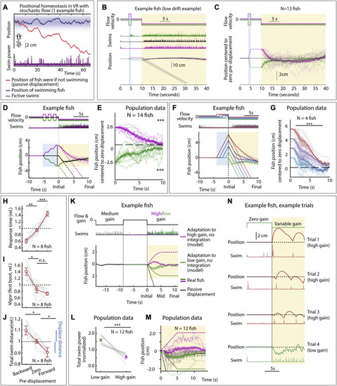
Positional homeostasis, extended characterization, related to Figure 1

(A) Positional homeostasis example, in which an example fish approximately stabilizes its location in a stochastic virtual water current.

(B) Positional homeostasis assay with a 30-s swim period in an example fish.

(C) Centered trajectories for N = 13 fish showing persistent convergence.

(D) Triple forward pre-displacement/backward pre-displacement assay. Example fish, showing converging trajectories, indicating successful integration across three consecutive pre-displacements. (Shaded regions: SEM in all panels.)

(E) Population data (14 fish) showing near-complete correction for earlier pre-displacement. (One-sample t test, ^∗∗∗p < 0.001, p = 9.7e−10 for forward pre-displacements, p = 1.9e−10 for backward pre-displacement. Error bars: SEM in all panels.)

(F) Assay to test integration over varying durations. An example fish successfully integrates pre-displacement and corrects for it in the swim period.

(G) Population data (4 fish) showing accurate correction, i.e., path integration. (Two-tailed paired t test, ^∗∗∗p < 0.001, p = 1.08e−7 for all forward pre-displacements.)

(H) Animals respond faster (slower) after a backward (forward) pre-displacement, consistent with Figure 1F. (Two-tailed paired t test, ^∗∗p < 0.01, p = 1.76e−3 for backward pre-displacement, ^∗∗∗p < 0.001, p = 3.1e−4 for forward pre-displacement.)

(I) Animals respond more vigorously after a backyard pre-displacement, consistent with Figure 1F. (Two-tailed paired t test, ^∗p < 0.05, p = 0.0151 for backward pre-displacement, n.s. p > 0.05, p = 0.115 for forward pre-displacement.)

(J) Total swim distance (normalized) corresponds to the earlier pre-displacement, consistent with Figure 1F. (Two-tailed paired t test, ^∗p < 0.05, p = 0.031 for backward pre-displacements, and p = 0.012 for forward pre-displacements.)

(K) After motosensory gain changes (high: ×1.5, low: ×0.5), animals still integrate position. Dashed lines: position of model fish performing gain adaptation (linear adjustment of vigor over 5 s) but no path integration. Solid lines: position of real fish.

(L) Swim vigor during low or high motosensory gain shows gain adaptation. (Two-tailed paired t test, ^∗∗∗p < 0.001, p = 1.6e−5.)

(M) Average fish position in low versus high gain trails initially diverges, then converges. Dashed lines: normalization to model fish performing gain adaptation but no path integration.

(N) Example trials during high and low motosensory gain (data from K–M) showing accurate positional homeostasis in both cases.

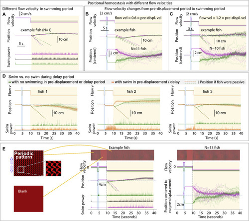
Additional features of positional homeostasis, related to Figure 1

(A) Trajectories of an example fish swimming against different flow velocities in the swim period.

(B and C) Behavior when flow velocity in the swim period is lower or higher than that in the pre-displacement period.

(D) Swimming in the pre-displacement or delay periods does not influence eventual fish location, i.e., fish track the visual stimulus and use integrated visual flow.

(E) Stimuli used to test if visual flow is sufficient for positional homeostasis. The periodic pattern looks the same when translated by an integer number of finely spaced periods. During the pre-displacement period, the fish transitions an integer number of periods. In the delay period, the screen becomes blank to additionally test whether animals are locking on to a specific feature of their environment. In the swim period, the pattern becomes visible again. Single-fish and population data shows convergence, i.e., positional homeostasis can be based only on integrated visual flow.

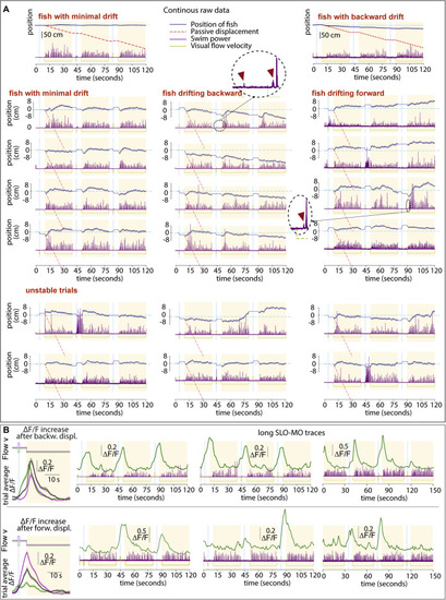
Examples of single, non-averaged trials, related to Figure 1

(A) Trajectories of three example fish (see Figure S4A for average trajectories of those and other fish). Trials are consecutive in groups of three, stacked vertically. For visualization, the start of the first of each triplet is shifted to zero. Little fictive “probe swims” are visible and magnified in the dashed circles; these probe swims are often present right after the start of a backward pre-displacement and at the start of swim periods and may inform the fish that it’s in an open-loop (pre-displacement) or closed loop (swim) period. We hypothesize that the probe swim in the pre-displacement may reduce subsequent swim attempts in the pre-displacement and delay periods, whereas in the swim period it may enhance further closed-loop swimming. In these fish, slow drift is present that can be minimal (left fish), backward (middle fish), or forward (right fish), i.e., positional homeostasis is not perfect. Figure S4A quantifies this drift and Figures S4B–S4F proposes an explanation in a control theory framework. The lower two rows illustrate “unstable trials,” showing that swimming behavior is variable and likely driven not only by visual flow but also other factors (e.g., fluctuating “internal states,” “noise,” etc.).

(B) Single-trial SLO-MO activity traces during 6.5 min of data for two example neurons with different tuning properties in one fish.

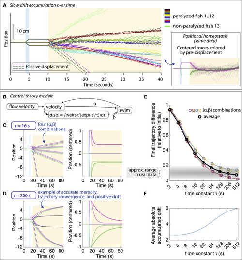
Drift in positional homeostasis and PID control theory, related to Figure 1

(A) Average trajectories showing drift in the swim period that can be slowly forward or slowly backward or minimal. Fish were not imaged. When fish were imaged and exposed to blue light-sheet laser light, drift tended to be larger. One unparalyzed fish was tested; this fish drifted forward. Despite the drift, average trajectories converged for every fish; average trajectories are shown in the same color for each fish for each of the three possible pre-displacements, with the different pre-displacements shown in distinct colors in the inset and in Figure S1C.

(B) Diagram of PID control system (see STAR Methods). Swimming is modeled as a continuous variable, a weighted linear combination of a velocity term and a displacement term, and constrained to be non-negative. The displacement term is a leaky integral of fish velocity with memory time constant τ.

(C) Example trajectories during simulated behavior with τ = 16 s for four (α,β) combinations, shown as raw position (left) and centered to the no-displacement trajectory (right). For this short time constant, trajectories converge only about halfway.

(D) For a longer memory time constant τ = 256 s, trajectories converge much more. Importantly, trajectories can drift forward or backward despite the fact that positional memory is quite accurate.

(E) For the four (α,β) combinations, the final trajectory difference is mainly a function of the memory time constant. In the real data, trajectories converge within about 5%–20%, suggesting a memory time constant of about a minute or more (gray shaded area).

(F) The average accumulated absolute drift over (α,β) pairs.

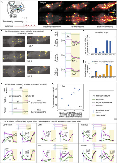
Positional homeostasis activity and variability, related to Figure 2

(A) Brain activity averaged over trials in an example fish shown as changes over time (ΔF/F)_t-1 and (ΔF/F)_t. Left: in the 300 ms following onset of backward flow through VR (forward visual motion from the point of view of the fish). Middle: at an intermediate time, after stimulus onset, just before (0–300 ms) swim onset. Right: immediately following (0–300 ms) swim onset.

(B) Examples of functional brain maps for individual fish before combining them into the final map in Figure 2D.

(C) With a 5 s delay period, fish perform positional homeostasis with little variability.

(D and E) Percentage of neurons dropped from each animal was small, and that the majority of these neurons resided in the forebrain.

(F and G) With a 17 s delay period, the number of SLO-MO neurons encoding the displacement memory appears to correlate to positional homeostasis performance, although the sample size is too small to be significant.

(H) Persistent positional encoding signals were detected in different brain regions, cerebellum, dorsal raphe nucleus, area of the interpeduncular nucleus, habenula, and pallium.

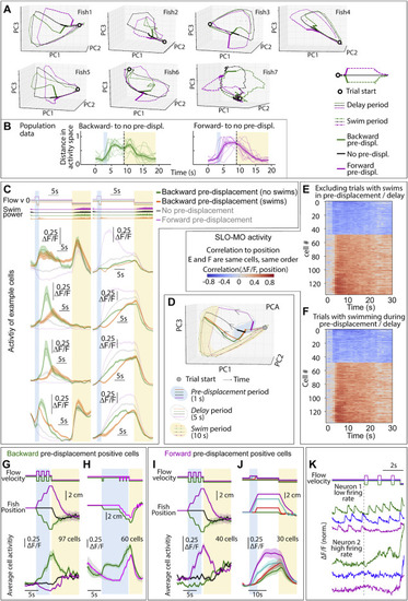
Further characterization of SLO-MO activity, dependence on complex trajectories and swimming, related to Figure 3

(A) Trajectories through dimensionally reduced network space for seven individual fish, related to Figure 3. Dimensionality reduction done with principal-component analysis (PCA).

(B) Distance in PC space (first 3 components) between backward pre-displacement and zero pre-displacement, and forward pre-displacement and zero pre-displacement activity, for 9 fish. Since distances are zero or greater, noise causes distance to always be positive even before the pre-displacement at ∼2 s. (Shaded regions: SEM.)

(C and D) SLO-MO cells showed a transient decrease in activity during swimming, after which they returned to activity levels encoding past displacements.

(E and F) Ranked correlation of cell activity to fish position for example fish of Figures 3B and 3C separated by trials with and without swimming in pre-displacement and delay periods.

(G) Neurons (in an example fish) with increasing activity following three consecutive backward or forward pre-displacements, showing integration. (Shaded regions: SEM in all panels.)

(H) Neurons (in an example fish) showing integration over backward pre-displacements. The green trials are offset by one additional displacement 5 s before the triplet displacement; this is reflected in a persistent increase in neuronal activity.

(I) Integration across triplet displacements by neurons that respond positively to forward displacements.

(J) Additional example of integration by SLO-MO neurons during forward pre-displacements of varying durations followed by delay periods.

(K) Individual neuron traces showing integration across triplet pre-displacements, fast imaging of single planes at 33 Hz. The firing rate of neuron 1 is low enough that individual spikes are visible in the calcium trace, showing persistently increasing spike rate after backward pre-displacements and persistently decreasing spike rate after forward pre-displacements. The firing rate of neuron 2 appears to be higher and, although individual spikes are not visible due to sampling rate and calcium indicator limitations, firing rate can be seen to increase following a backward pre-displacement relative to a forward pre-displacement.

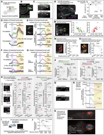
Additional ablation and stimulation results, and dorsocaudal hindbrain anatomy, related to Figures 2, 5, and 6

(A) Ablation setup for ablating functionally identified SLO-MO populations using a two-photon laser and Tg(elavl3:GCaMP6f) fish.

(B and C) Calcium imaging of functionally identified and targeted SLO-MO cells before and after two-photon ablation showing single-cell precision.

(D) SLO-MO cells (of one example fish) whose activity increases after backward pre-displacement, before and after ablation of SLO-MO cells whose activity increases after forward pre-displacement. A sensory response remains, but persistence is abolished.

(E) Population data, similar to (D), showing the loss of persistent activity but preservation of sensory responses across 3 fish. Inset: example single imaging plane showing some spatial intermingling of forward-tuned SLO-MO cells (magenta) and backward-tuned SLO-MO cells (yellow).

(F and G) Similar to (D) and (E), but showing activity of forward-tuned cells before and after ablation of backward-tuned cells, again showing the loss of persistence but preservation of sensory responses.

(H) Additional quantification of the effects of SLO-MO ablation. Ablation of backward-tuned cells, ablation of forward-tuned cells, and control ablations are shown. (Two-tailed paired t test, ^∗∗p < 0.01, ^∗p < 0.05, n.s. p > 0.05. Error bars: SEM in all panels.)

(I) Diagram of optogenetic stimulation and functional imaging setup.

(J) Optogenetic excitation of functionally identified SLO-MO neurons causes changes in the time to first swim bout in the swim period, consistent with changes in distance swum shown in Figures 5G and 5H. (Two-tailed paired t test, ^∗∗∗p < 0.001.)

(K) Functionally identified SLO-MO neurons in Tg(gad1b:Gal4; UAS:CoChR; elavl3:jRGECO1b) fish from the elavl3:jRGECO1b red channel overlaid with the gad1b:Gal4; UAS:CoChR green channel. Single-cell specificity is obtained by sparse expression of CoChR (using the Gal4-UAS system) and stimulation with a high-resolution DMD setup.¹²³

(L) Optogenetic stimulation of SLO-MO neurons (one neuron at a time of any functional type; hence no significant integration expected) causes inhibition of specific IO neurons (population data). Stimulation of CoChR-positive non-SLO-MO neurons causes no significant IO response. (p = 1.7e−7 by one-way ANOVA, 9 fish. ^∗∗∗p < 0.001, by Tukey’s post hoc test. Same data as Figure 2K. Shaded regions and error bars: SEM in all panels.)

(M) Correlation between lateral and medial IO activity and reaction time, complementing the joint decoder of Figure 6G.

(N and O) Backward displacements suppress medial IO activity; forward displacements suppress lateral IO activity. Population data to complement Figures 6A–6D. (One-sample t test, ^∗∗∗p < 0.001.)

(P) Additional quantification of effects of IO lesions on response time and swim power. (9 fish, two-tailed paired t test, ^∗∗∗p < 0.001, ^∗p < 0.05. Error bars: SEM in all panels.)

(Q) Calcium imaging of IO neurons using Tg(elavl3:H2B-GCaMP6f) fish before and after IO ablation.

(R) Persistent SLO-MO activity encoding self-location remains intact after ablation of IO cells.

(S) Known and hypothesized neuroanatomy of the dorsocaudal larval zebrafish hindbrain. This schematic, based on multiple zebrafish and mouse publications and atlases, accompanies the hypothesis that SLO-MO overlaps with the homolog of the nucleus prepositus hypoglossi (NPH), a major GABAergic input to the IO.^94,95 SLO-MO neurons are also GABAergic and project to and inhibit the IO. Our results are consistent with a monosynaptic connection between SLO-MO and IO, and we showed that activating SLO-MO functionally inhibits IO. SLO-MO neurons are spatially arranged relative to the nucleus of the solitary tract (NTS), noradrenergic area A2⁹⁶ (called NE-MO in Mu et al.⁵²), and are close to the fourth ventricle ⁹⁷; the NPH also has these properties (Allen Mouse Brain Atlas, ⁹³). Historically, the NPH has been studied in the context of eye movement control, but (parts of) the NPH may be multifunctional. Circuits for positional homeostasis and for oculomotor control have in common that they must integrate visual slip into a persistent signal,^{124, 125, 126},so the possibility exists that these circuits showed some overlap, possibly with similar mechanisms for persistent activity.