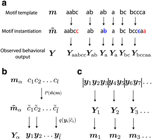
a) Motif templates are fixed sequences of elementary locomotor episodes (labeled a, b and c in this example). The observed behavioural output is generated from motif templates drawn sequentially from a dictionary. An instantiation of a template may “mutate” by insertions (red) or deletions (blue), which then generates the observed output as shown in panel (b). (b) The generative process from a motif template c₁ c₂…c_l to instantiation to observed output. c) The unsupervised inference procedure (BASS) first learns a dictionary of motifs and then segments (vertical bars) the observed behavioural output y₁, y₂, … into the most likely sequence of motifs m₁, m₂, … from the dictionary that generated it.

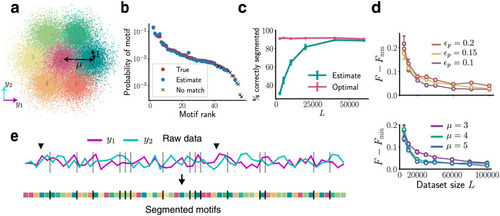
BASS accurately identifies and segments motifs in noisy, synthetic data: (a) The seven clusters from which the two-dimensional data (along y₁, y₂) is drawn. (b) The true probabilities of the motifs (red dots) and probabilities estimated (blue dots) by our algorithm showing successful reconstruction of the dictionary. The crosses are low-probability motifs not identified by the algorithm (see main text). (c) The percentage of correct segmentations into motifs (cyan) with increasing dataset size. The optimal percentage when the true dictionary is known is shown in pink. In panels b,c and e, we use L = 40000, ϵ_p = 0, ϵ_b = 0.5, μ = 3. See S1 Fig for the case ϵ_p > 0. (d) The difference in the negative log-likelihood per symbol after convergence when the true dictionary is unknown (F) and known (F_min). Action pattern noise ϵ_p and locomotor episode noise μ are successfully integrated out with larger datasets. Top: μ = 3, p_d = 0.5, Bottom: ϵ_p = 0.15, p_d = 0.5, where p_d is the probability of a deletion in a motif instantiation. Error bars are s.e.m. (e) A snippet of the raw data sequence and the most likely partitioning into motifs found by the algorithm. The vertical bars delineate two successive motifs. The black arrows mark two instantiations of the same length-five motif.

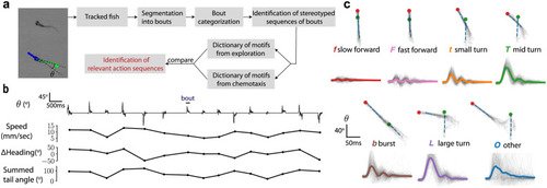
(a) Overview of the analysis pipeline. (b) A time series of the tail angle θ shows the discrete nature of locomotor episodes (‘bouts’) with the corresponding speed, change in heading and the summed tail angle calculated as the summed absolute amplitude of the tail angle. (c) Samples of the seven bout types identified using a Gaussian Mixture Model. In the superimposed images corresponding to a given bout type, the green and red dots correspond to the head position at the bout beginning and end respectively. Below each sample, the average tail angle θ is shown in solid color with 200 trajectories shown in grey.

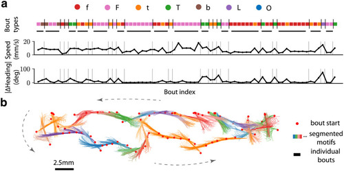
(a) A sample sequence of 75 bouts from the exploratory data segmented (separated by vertical bars) into the most likely sequence of motifs from the learned dictionary. The corresponding speed and absolute change in heading are shown. Motifs longer than one locomotor episode are underlined in gray. (b) A sample trajectory consisting of 80 bouts (head position at the beginning of a bout is shown as a red dot) are segmented into motifs (head and tail at each frame are shown), where successive bouts from the same motif have the same color. The black-colored segments of the trajectory are motifs of length one i.e., single locomotor episodes.

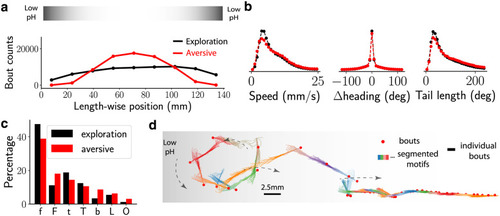
(a) Histogram of larvae positions along the well with and without the aversive (acidic) gradient, located at the ends of the well. The s.e.m is square-root of the counts, which is negligible. An illustration of the aversive gradient is shown above. (b) The distribution of speed, change in heading and the summed tail angle of all bouts during exploration (black) and in aversive environment (red). The difference in global kinematic parameters between the two environments is small. (c) The fraction of each bout type in exploratory and aversive environments, where a total of ≈ 85000 and ≈ 66000 bouts were collected respectively, shows an increase in fast bouts: b,F and O. (d) Localisation of bout types along the well with and without the aversive (acidic) gradient, (e) BASS segments a series of bouts from the aversive environment into sequence of recurring motifs. Shown here is a sample trajectory (as in Fig 4b) where the fish escapes from the aversive environment.

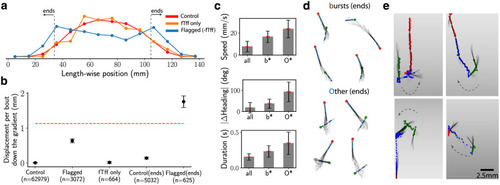
(a) Distributions of length-wise positions for the Control bouts (all bouts from aversive environment except the ones from sequences flagged as over-represented in Table 2), fTff only and Flagged bouts (from the sequences in Table 2) except fTff in red, orange and blue respectively. (b) The length-wise displacement travelled in a bout down the gradient for bouts tagged as Control, Flagged (as defined in (a)), fTff only, Control(ends) (all bouts from the two ends of well shown in (a)), Flagged(ends) (flagged but with fTff removed and in the ends of the well). For scale, the red, dashed line shows the mean length-wise distance per bout for unflagged bouts. Error bars are s.e.m. (c) The mean speed, change in heading and duration of the bouts (black, red error bars for s.d, s.e.m respectively) from b and O bout types that are part of the Flagged(ends) sequences from (b). (d) Superimposed images for four random samples of b and O bout types from the flagged sequences in (a). The green and red are the head positions at the beginning and end of the bout respectively. (e) Superimposed images for four random samples highlighting the Flagged(ends) sequences (blue dots), which include the three bouts before (green dots) and after (red dots) the flagged sequence. Note that the depicted gradient is illustrative.

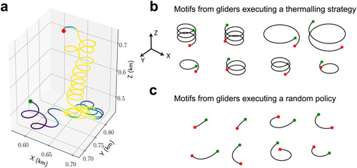
(a) A sample trajectory showing the thermalling behaviour of the soaring glider. The glider reacts to mechanical cues such as torques and accelerations. See [25,26] for more details. Regions of downdraft and updraft (blue through yellow) are marked, which highlight the relatively disperse trajectories in downdrafts compared to the spiraling behaviour in updrafts. (b) Motifs found by BASS that span the largest fraction of the thermalling dataset (i.e., episodes where the glider used a thermalling strategy). Most enriched motifs are those of a spiralling pattern. The green and red dots mark the start and end points. Note that the glider sinks without updrafts. (c) Same as (b) for motifs found in the dataset of a glider executing a random policy