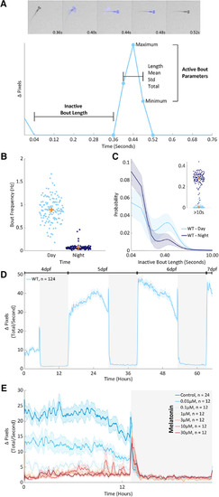
Behavior at scale. A, top panel, Five consecutive frames from an individual well of a 96-well plate as a 6 dpf zebrafish larva performs a swim bout. Blue highlights pixels that change intensity between frames (Δ pixels). Lower panel. A Δ pixels time series from the larva above. Highlighted are the features that describe each active and inactive bout. B, Mean bout frequency (Hz) recorded from individual larvae at 5 and 6 dpf during the day (light blue) and the night (dark blue). Each dot is 1 of 124 wild-type larvae. The orange crosses mark the population means. C, The probability of observing different lengths of inactivity during the day (light blue) or the night (dark blue) at 5 and 6 dpf. Each larva’s data were fit by a pdf. Shown is a mean pdf (bold line) and SD (shaded surround) with a log scale on the x-axis cropped to 10 s. Inset, The total probability of inactive bout lengths longer than 10 s, per animal. D, The mean activity of 124 wild-type larvae from 4 to 7 dpf, on a 14/10 h light/dark cycle. Data for each larva was summed into seconds and then smoothed with a 15-min running average. Shown is a summed and smoothed mean Δ pixels trace (bold line) and SEM (shaded surround). E, Average activity across one day (white background) and night (dark background) for larvae dosed with either DMSO (control) or a range of melatonin doses immediately before tracking at 6 dpf. Data were summed and smoothed as in D. The number of animals per condition is denoted as n. Extended Data Figures 1-1, 1-2, 1-3 support Figure 1.

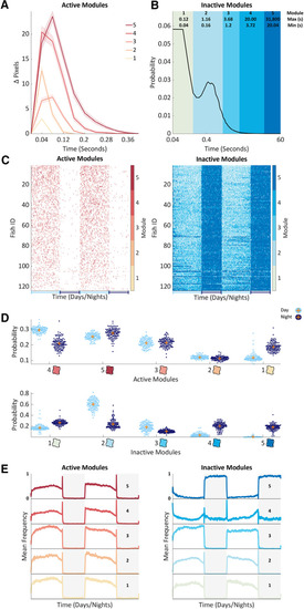
Unsupervised learning identifies contextual behavioral modules. A, Average Δ pixels changes for each active module. Shown is the mean (bold line) and SEM (shaded surround) of 100 bouts randomly sampled from each module from one representative larva. Modules are numbered and colored by average module length across all animals, from shortest (1) to longest (5). B, A probability density curve showing the distribution of inactive bout lengths in seconds, on a log x-axis cropped to 60 s. Modules are numbered and colored from shortest (1) to longest (5) mean length (see legend for each module’s minimum and maximum bout length). C, Matrices showing the active (left) or inactive (right) module assignment of every frame (x-axis) for each of 124 wild-type larvae (y-axis) across the 14-h days (light blue underlines) and 10-h nights (dark blue underlines) from 5 to 6 dpf. Larvae were sorted by total number of active modules from highest (top) to lowest (bottom). Modules are colored according to the adjacent colormaps. D, Average active (upper) and inactive (lower) module probability during day (light blue) and night (dark blue) 5 and 6 of development. Each of 124 wild-type animals is shown as a dot and orange crosses mark the population means. Active modules are sorted by mean day probability from highest to lowest (left to right). Inactive modules are sorted by mean length from shortest to longest (left to right). The blobs correspond to the color used for each module in other figures. E, The mean frequency of each active (left) and inactive (right) module across days 5 and 6 of development. Shown is a mean smoothed with a 15-min running average, rescaled to 0–1. Days are shown with a white background, nights with a dark background. Modules are sorted from shortest to longest (lower to upper panels). Extended Data Figures 2-1, 2-2 support Figure 2.

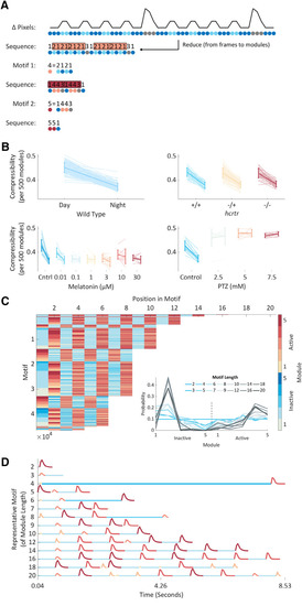
Hierarchical compression reveals structure in zebrafish behavior. A, Compression explained using fictive data. Top to bottom, From Δ pixels data (black trace), we classified both active and inactive behaviors into modules (colored circles). From modular behavioral sequences, we identified motifs (sequences of modules) using a compression algorithm. Compression iteratively identifies motifs (shown as boxes) by replacing them with new symbols until no more motifs can be identified and the sequence is maximally compressed. B, Each panel shows how compressibility, calculated from 500 module blocks, varies in different behavioral contexts. Each pale line shows an individual fish’s mean compressibility during the day and the night. The darker overlay shows a population day and night mean ± SD. In the wild-type data, compressibility is higher during the day than the night (p < 10⁻¹⁵⁸) and increases from day/night 5–6 (p < 10⁻⁴), findings consistent across triplicate experiments. Melatonin decreases (p < 10⁻¹⁰), while PTZ increases compressibility (p < 10⁻⁸). There is no effect of hcrtr genotype on compressibility. Statistics are two-way or four-way ANOVA. C, All 46,554 unique motifs (y-axis) identified by compressing data from all animals. Each motif’s module sequence is shown, with the modules colored according to the colormap on the right. Motifs are sorted by length and then sequentially by module. Motifs range in length from 2 to 20 modules long. Inset, For each motif length, the probability of observing each inactive or active module. D, Each motif in the library consists of an alternating sequence of Δ pixels changes and pauses (active and inactive modules). A representative motif of each module length is shown with each module colored according to the colormap in C. Representative motifs were chosen by determining every motif’s distribution of modules and then for each observed module length, selecting the motif closest to the average module distribution (see C, inset). Extended Data Figure 3-1 supports Figure 3.

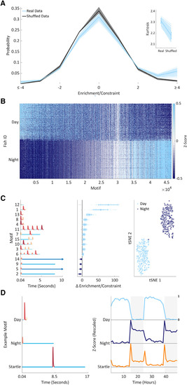
Supervised learning identifies contextual behavioral motifs. A, pdfs showing the probability of observing motifs at different enrichment/constraint scores rounded to whole numbers and summed at values above or below ±4 for ease of visualization. Each wild-type animal is depicted by a single pale blue (real data) and 10 black (shuffled data) lines; overlaid in bold are mean pdfs. The inset shows that the kurtosis of the real data are higher than the shuffled data (p < 10⁻²⁷¹; two-way ANOVA, real vs shuffled data, no significant interaction with experimental repeat factor). Each larva is shown as a pale line; overlaid is a population mean and SD. B, Enrichment/constraint scores for all 46,554 motifs (x-axis) for each fish during day/night 5 and 6 of development (y-axis). To emphasize structure, motifs are sorted in both axes, first by their average day/night difference (from day to night enriched left to right), then separately day and night by larva. Finally, each motif’s enrichment/constraint score is Z-scored to aid visualization. C, left, The 15 day/night mRMR motifs module sequences are shown numbered by the order in which they were selected by the algorithm. Motifs are sorted by day minus night enrichment/constraint score (middle). The long pauses at the end of motifs 5 and 14 are cropped at 10 s (arrows). Middle, For each selected motif (y-axis), ordered as in the left panel, each wild-type animal’s (124 in total) day minus night enrichment/constraint score (x-axis) is shown as a dot. Values above zero are colored light blue; below zero are dark blue. Overlaid is a population mean and SD per motif. Right, A tSNE embedding of the 15-dimensional motif data (middle) into a two-dimensional space. Each circle represents a single day (light blue) or night (dark blue) sample. D, Representative motif temporal dynamics; shown are motifs 1 (day) and 2 (night) from C, as well as a startle-like motif. Left, Each motif’s module sequence. Right, Each motif’s mean enrichment/constraint score each hour, rescaled to 0–1. Extended Data Figure 4-1 supports Figure 4.

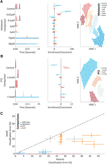
Pharmacological behavioral motifs. A, left, Module sequences for the single best motif for each melatonin comparison. Modules are colored as elsewhere. Middle: for each dose’s single best motif, see left panel y-axis for dose, enrichment/constraint scores are shown for every dose on a log x-axis. Each animal is shown as a dot, with a mean ± std overlaid per dose. Right, A two-dimensional tSNE embedding from a space of 912 unique motifs. Each animal is shown as a single dot underlaid by a shaded boundary encompassing all animals in each condition. B, left, Module sequences for the single best motif for each PTZ comparison. To highlight a seizure specific motif, the control motif and corresponding enrichment/constraint score shown is mRMR motif 2, not 1, for this comparison. Modules are colored as elsewhere. Middle, For each dose’s single best motif, enrichment/constraint scores are shown for every dose on a linear x-axis. Each animal is shown as a dot, with a mean and SD overlaid per dose. Right, A two-dimensional tSNE embedding from a space of 338 unique motifs. Each animal is shown as a single dot underlaid by a shaded boundary encompassing all animals in each condition. C, Each classifier’s classification error (%) is shown in terms of modules (x-axis) and motifs (y-axis). Data are shown as mean and SD from 10-fold cross validation. Classifiers are colored by experimental dataset (see Legend). For reference, y = x is shown as a broken black line. Data below this line demonstrates superior performance of the motif classifiers.