Setup and circuit overview. a Simplified circuit schematic for horizontal eye movements. Red dashed rectangle represents imaged brain area; blue cones show location of Mauthner cells. ABN, abducens nucleus; B, burst neurons; Dien, diencephalon; INN, internuclear neurons; IO, inferior olive; LR, lateral rectus; MB, midbrain; MN, motoneurons; MR, medial rectus; OMN, nucleus oculomotorius; OI, oculomotor integrator; PT, pretectum; rh 4–8, rhombomeres 4–8; VSM, velocity storage mechanism; Θ, eye position. Note that the connection from the VSM to the ABN in zebrafish is probably indirect [7]. Dashed arrows indicate direct or indirect inputs from upstream visual brain areas [8, 9]. a’ Simplified schematic response profiles for hindbrain oculomotor neurons during eye position changes. Dashed line represents an eye position or velocity of 0. L, left; P_L/R, Position coding neurons left/right, note that P_L and P_R have different firing thresholds; R, right; V_F, fast (burst) velocity neurons; V_S, slow velocity neurons. b Schematic of microscopy setup. Agarose-embedded zebrafish larvae were visually stimulated, while eye movements were recorded from below, and cellular calcium signals were recorded from above via a two-photon microscope. Setup not drawn to scale, binocular zone excluded for experiment with monocular stimulation only, scale bar 50 μm, red dashed rectangle represents imaged brain area, red arrows show GCaMP expression in the nuclei of the Mauthner cells, which served as a landmark (blue cones in a and in cell maps). A, anterior; L, left; P, posterior; PMT, photomultiplier tubes; R, right

Experimental strategy to assess binocular coordination. a: Example stimulus protocol (from recording shown in a’). Lines indicate direction in which the stimulus is moving. Dashed lines separate stimulus phases. a′ Example eye traces (right eye (RE): magenta, left eye (LE): cyan) and corresponding neuronal calcium responses (black, ΔF/F) with monocular coding. The respective highest scoring regressor [monocular right eye, rightward eye position (r3); monocular left eye, rightward eye position (r7)] is shown in blue. Grey line shows right eye position from which r3 was derived. b Example eye traces with derived binocular regressors (top 3 plots) and calcium responses of binocular neurons in the same recording (lower 2 plots). Left and right eye traces with capped counter-clockwise eye velocity (grey, upper two plots) and averaged eye position (grey, third plot) of which regressors 18 (binocular always leftward position, blue trace in third and fourth plot) and r24 (binocular always leftward velocity, blue trace in fifth plot) were derived. Black lines show ΔF/F (DFF) calcium signals for a binocular always (BA) position (P) and a BA velocity (V) neuron with the corresponding highest scoring regressor in blue. b′ Example binocular preferred (BP) position neuron with respective eye trace; note the binocular event during the LE stimulation (red arrow). The blue trace shows the respective regressor (binocular preferred, rightward position, r1), the red trace the corresponding velocity regressor (binocular preferred, rightward velocity, r9). c Overview of kinematic eye parameters addressed in this study to classify response types and regressor overview. Left, depiction of kinematic parameters. Middle, response types. Each set of three squares corresponds to one type of regressor, see colour legend. Right, full list of regressors in grey. Italic numbers correspond to averaged regressors; BE, both eyes; MLEX, monocular left eye exclusive; MREX, monocular right eye exclusive

Monocular and binocular cell maps. a–d Transversal, sagittal, and dorsal views for MRE and binocular neurons in the hindbrain (see Additional file 1: Figure S1a-b for mirror-symmetric MLE neurons). Pooled neurons in each figure had the highest correlation to the appropriate regressors mentioned in the legend. A, anterior; ABN, abducens nucleus; BA, binocular always; BP, binocular preferred; D, dorsal; L, left; M, Mauthner cells; MRE, monocular right eye; P, position/posterior; R, right; r, regressor; rh 5-8, rhombomeres 5-8; V, ventral/velocity; each coloured ball represents one neuron identified in one fish. Shaded areas in subfigure a show the location of motoneurons expressed in the transgenic Tg(mnx1:TagRFP-T)vu504Tg line (mean vertices position plus standard deviation of three 5 dpf old fish). Sparse, single labelled neurons in the dorsal region have not been highlighted [34]

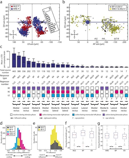
Monocular/binocular synopsis. a Transversal projection of monocular coding neurons within rh5/6 (ABN). D, dorsal; L, left; M, Mauthner cells; MLE, monocular left eye; MRE, monocular right eye; P, position; R, right; V, ventral. Black arrows indicate position of a faint gap between the ventral and dorsal clusters of putative internuclear neurons. Inset shows the numbers of neurons plotted in this figure for the left hemisphere along the D-V axis rotated by 20°. b Monocular and binocular velocity encoding neurons. A, anterior; BA, binocular always; BP, binocular preferred; P, posterior; rh 5-8, rhombomere 5-8; V, velocity. Black arrow indicating the direction of the velocity shift. c Sum of the total number of neurons found for each response type sorted pairwise according to the affected muscle(s). The bar plot shows the mean and standard deviation for eight composite brains. BA, binocular always; BP, binocular preferred; MLE, monocular left eye; MLEX, monocular left eye exclusive; MRE, monocular right eye; MREX, monocular right eye exclusive. d Monocular coding differences for all four main response types for position coding neurons. Index running from − 1 (exclusively coding for left eye) to + 1 (right eye). e PV influence for BA P and BP P neurons. Index running from − 1 (exclusive velocity influence) to + 1 (exclusive position influence). f, g Left and right eye firing thresholds acquired during the firing threshold analysis pooled in ON direction

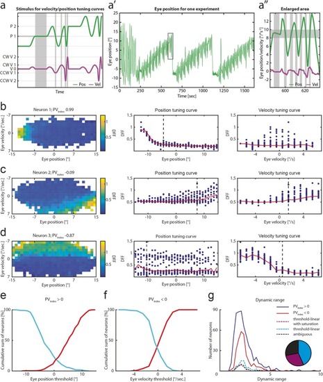
Neuronal tuning for eye velocity and position. a Schematic of the closed loop velocity/position stimulus for highlighted eye position (P1) at different slow-phase eye velocities (CCW V2, CCW V1, V0, CW V1, CW V2). Only two velocity steps are depicted for illustration purposes. Grey shaded rectangles show one eye position bin and different velocities for that bin. CCW, counter-clockwise; CW, clockwise; P, position; V, velocity. a′ Example binocular eye trace for one recording. a″ Highlighted area from a′. Grey boxes as in a. b–d Left panel, tuning curves showing DFF colour coded for averaged eye position-velocity bins. Middle panel, position tuning curve. Red line shows averaged DFF between ± 1°/s eye velocity; blue dots for every other eye velocity bin (as in left panel). A black dashed line shows the firing threshold, if identified. Right panel, same as for the middle panel, but for eye velocity. Red line shows averaged DFF between ± 1° eye position. e Cumulative position threshold plot for position coding neurons (PV_Index > 0) pooled in ON direction to the right (red, n = 250) and left (cyan, n = 283). f Cumulative velocity threshold plot for velocity coding neurons (PV_Index < 0) pooled in ON direction to the right (red, n = 104) and left (cyan, n = 175). g Dynamic range of fluorescence for position and velocity coding neurons (PV_Index > 0, PV_Index < 0 respectively) and for neuron with a very strong velocity coding (PV_Index < − 0.5, dashed lines) separated by their response profile. Pie chart showing the relative numbers for strong velocity coding neurons (w/ saturation, 29% (40/139); w/o saturation, 43% (60/139); ambiguous, 28% (39/139))

PV_Index distribution and spatial location of identified neurons. a–c Sagittal (a), dorsal (b), and transversal (c) anatomical views of eye-correlated neurons colour-coded for the PV_Index which was calculated from the closed-loop experiment. Histograms show the anatomical distribution of neurons along the appropriate axis for either all neurons or exclusively for rh7/8. Blue cones, Mauthner cells; blue line, MLF; A, anterior; D, dorsal; L, left; P, posterior; R, right; V, ventral; error bars are SEM

Summary for binocular coordination and PV encoding in the larval zebrafish hindbrain. a Anatomical separation of monocular and binocular neurons in the dorsal view. For illustrative purposes, all monocular domains are depicted in the right hemisphere, and binocular domains in the left hemisphere (no difference across hemispheres was identified). A, anterior; L, left; M, Mauthner cells; P, posterior; R, right; rh5-8, rhombomere 5-8. b Distinct clusters of eye movement coding neurons in the hindbrain (side view). Arrows indicating position-velocity shift in the OI. D, dorsal; V, ventral. c Schematic illustrating each response type. Note the absence of slow-phase velocity neurons with preferred binocular (BP) encoding and the lack of monocular neurons for the temporal half of the ipsilateral eye outside of the nucleus abducens. Dashed lines represent “missing” neuronal clusters, i.e. only a small numbers of neurons were found for the respective eye movements