
- Title
-
Bayesian inference of neuronal assemblies
- Authors
- Diana, G., Sainsbury, T.T.J., Meyer, M.P.
- Source
- Full text @ PLoS Comput. Biol.
(A) Simulated activity of |
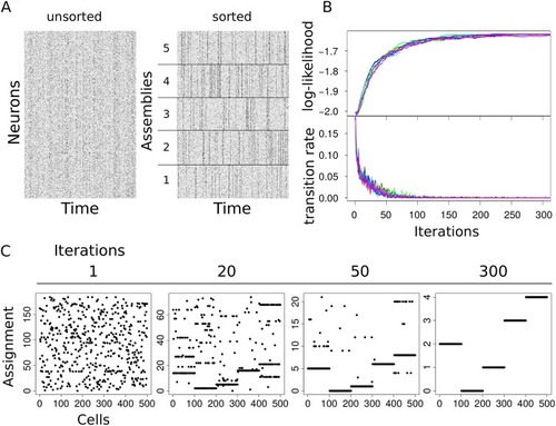
(A) Simulated activity of |
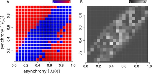
The ability to identify assemblies in a dataset depends on the model parameters. When synchrony and asynchrony levels are too similar, the recording time might not be sufficient to capture small differences in firing patterns. (A) Raster plot displaying detectable (red) versus non-detectable (blue) regimes of as a function of synchrony and asynchrony parameters of the model (we used 5 randomly generated assemblies for each configuration of synchrony and asynchrony). (B) Raster plot representing the number of neurons reassigned, on average, for every random sample of the Markov chain. The average transition rate can be viewed as an order parameter characterizing the transition between detectable and non-detectable phases. |
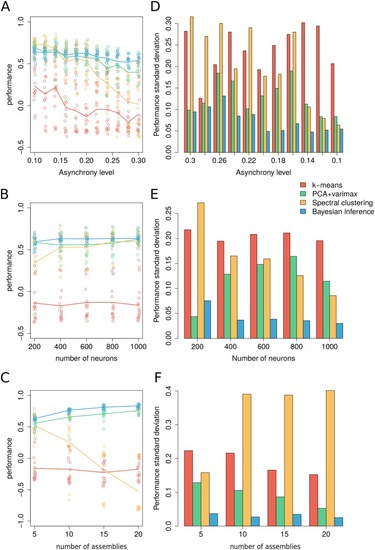
(A) Performance comparison across levels of asynchrony. Dots correspond to independently generated data sets while solid lines show the average performance for each method over all simulated data. (B) Comparison across number of neurons. (C) Comparison across number of assemblies. (D-F) Standard deviation of the performance across simulated data per parametric condition. Unless specified otherwise, surrogate datasets were generated using 400 neurons and 1000 time frames distributed over 5 assemblies with assembly activity of 5%, synchrony 50% and asynchrony 10%. For |
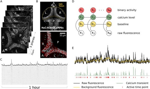
(A) Volumetric 2-photon imaging of both tectal hemispheres showing anterior/posterior (A/P) and right/left (R/L) axis of the zebrafish optic tectum. We monitored activity in the tectum of immobilized zebrafish larvae kept in total darkness. In all experiments we recorded calcium activity for 1 hour throughout 5 planes, 15 |
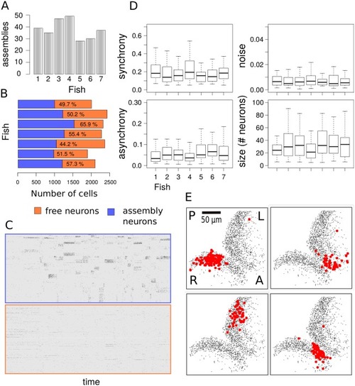
(A) Number of neuronal assemblies estimated for each fish. (B) Fraction of neurons assigned to assemblies with 99% confidence. The efficacy of our method in capturing neuronal assemblies is illustrated by separating the activity matrix of assembly neurons from neurons which are not part of a coherent assembly. (C) When sorting the activity matrix by membership, neurons that are part of an assembly generate bands of synchronous activity whereas neurons that are not assigned to an assembly display independent random firing events. (D) Comparison of synchrony, asynchrony, activity and assembly sizes for all experiments. Synchrony and asynchrony correspond to the model parameters λ(1) and λ(0), as the probabilities of a neuron to fire with its assembly (synchronous activation) and independently of it (asynchronous activation). The activity corresponds to the probability of an assembly to be active at any time during the 1 hour recording period. (E) Representative assemblies from single fish with high synchrony and activity display spatial compactness within left or right tectal hemispheres. Labels A/P and R/L indicate anterior/posterior axis and right/left optic tectum respectively. Assembly maps are obtained by projecting in 2D the positions of all member neurons across the five imaging planes. |
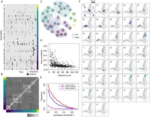
(A) Raster plot of assembly activity ordered according to subnetwork membership as shown in C. (B) Raster plot of the time correlation matrix (Pearson’s) between all pairs of assemblies averaged across posterior samples and sorted according to subnetwork membership. (C) Subnetwork graphs representing the time correlations among neuronal assemblies (see |
(A) 2D spatial distribution of neurons recorded from the mouse visual cortex from Ref. [ |

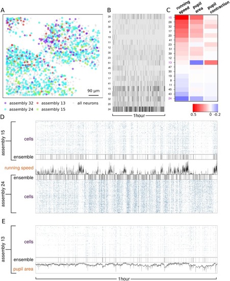
(A) Identification of exponentially decaying activity transients from spike counts using bin size of 0.6s. (B) Binary activity matrix obtained by combining transient events from 242 neurons. (C) Raster plot of the assembly activity. (D) Raster plot of the time correlation matrix between neurons sorted by assembly membership. (E) Time correlation between each assembly activity and the absolute wheel velocity. Boxplots represent the distribution of correlation across posterior samples. (F) Comparison between correlated and anti-correlated assemblies with respect to wheel motion. |