Ongoing activity and localized bursting in the optic tectum.

(A–B) Left: Pairwise activity correlation as a function of Euclidean distance between cells in two additional example fish (red shaded area denotes SD across cells, n=18,580 and 10,948). Middle: Example correlation maps alongside Gaussian and exponential fits for the same fish. Right: Positions of peaks of the fitted functions vs positions of seed cells. Spot colors indicate r² values. (C) Same analysis as A-B but for two-photon imaging of single plane in OT of a third fish. (D) To select the MinPts parameter for DBSCAN, we performed a shuffle analysis in which the time base for each neuron was circularly permuted. Plot shows the mean number of detected bursts across 10 permutations as a function of the MinPts parameter. Shaded area indicates SD, arrow indicates the conservative value we chose, where zero bursts were detected in shuffled data. (E) Bursts detected for one tectal activity peak for different values of MinPts. Rectangle indicates chosen value. A, anterior; P, posterior; Med, medial; Lat, lateral.

Ongoing activity and localized bursting in the optic tectum.

(A–B) Left: Pairwise activity correlation as a function of Euclidean distance between cells in two additional example fish (red shaded area denotes SD across cells, n=18,580 and 10,948). Middle: Example correlation maps alongside Gaussian and exponential fits for the same fish. Right: Positions of peaks of the fitted functions vs positions of seed cells. Spot colors indicate r² values. (C) Same analysis as A-B but for two-photon imaging of single plane in OT of a third fish. (D) To select the MinPts parameter for DBSCAN, we performed a shuffle analysis in which the time base for each neuron was circularly permuted. Plot shows the mean number of detected bursts across 10 permutations as a function of the MinPts parameter. Shaded area indicates SD, arrow indicates the conservative value we chose, where zero bursts were detected in shuffled data. (E) Bursts detected for one tectal activity peak for different values of MinPts. Rectangle indicates chosen value. A, anterior; P, posterior; Med, medial; Lat, lateral.

Stochastic spiking network model reproduces tectal bursting.

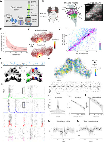
(A) LNP Model architecture: connection weights for excitatory (E) and inhibitory (I) interactions are determined by Gaussian functions of the intercellular Euclidian distance, with unique gain (g^(E),g^(I)) and spatial standard deviation (σ^(E),σ^(I))for each type of interaction. Presynaptic spikes are filtered in time with time constants (τ^(E),τ^(I))and summed along with a bias (μ) to produce the linear drive (excitability state). Exponentiating this linear drive sets the mean of an inhomogeneous Poisson process from which spikes are randomly emitted (Materials and methods). Model parameters used for all panels in this figure are shown inset. (B) Example of burst detection in the simulation results (c.f. Figure 1F)(C) Left: Locations of bursts detected during a 30 min simulation. Colors indicate burst times and spot sizes indicate number of participating neurons. Right: Burst locations vs. burst time. Rectangle widths indicate the temporal extent of each burst. (D–E) Neuronal assemblies detected using PCA-promax algorithm (Materials and methods), for simulation results (D) and experimental data (E), shown on a spatial map (top) and a raster plot for representative assemblies (bottom). (F) Time-course of linear drive to model cells around the time of a spontaneous burst (t=0). Star indicates burst centroid.

Exploration and optimization of model parameters.

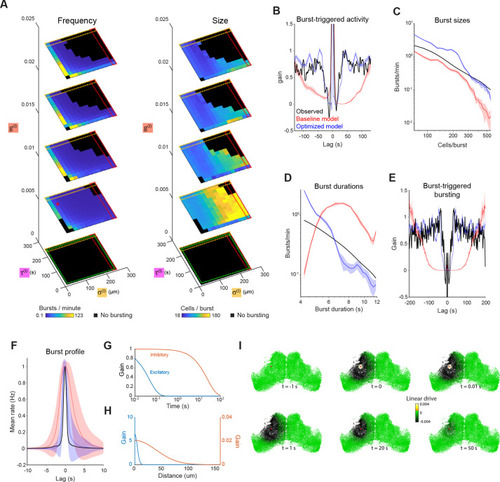
(A) Burst rate (left) and number of participating neurons (right) as a function of inhibitory space constant (σ ), inhibitory time constant (τ^(I)) and inhibitory gain (g^(I)). Red star indicates the parameters of the baseline model (as per Figure 2), and black regions indicate parameter combinations that failed to produce bursting. Dashed squares indicate regions approaching uniform inhibition (red), non-decaying inhibition (orange) and lack of inhibition (green). (B–D) Model simulation evaluated against optimization objectives: post-burst activity suppression (B), burst sizes distribution (C) and burst durations distribution (D). (E–F) Model simulation vs experimental data for two additional features: Burst-triggered burst participation (E, see Figure 1L) and burst temporal profile (F, see Figure 1H). (G–H) Temporal (G) and spatial (H) profiles of the intercellular interactions in the optimized model. (I) Timeseries illustrating the influence of a single spike (in cell marked with red spot) on the linear drive of surrounding cells in the optimized model network. Plots show mean and shaded areas indicate SD for n=10 simulation runs.

Model variations and optimization using EMOO.

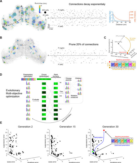
(A–B) Bursts produced in simulations where the connections decay in space according to an exponential function (A), and where 20% of the connections were randomly eliminated (B). Left: Locations of bursts detected during a 30 min simulation. Colors indicate burst times and spot sizes indicate number of participating neurons. Right: Burst locations vs. burst time. Rectangle widths indicate the temporal extent of each burst. (C) Top: the change in bursting characteristics following 10% and 20% random synaptic pruning (grey) could be compensated for by re-tuning the model parameters (using evolutionary multi-objective optimization, EMOO, see below). Bottom: model parameters before and after re-tuning. (D) Schematic of EMOO (evolutionary multi-objective optimization). In each generation, a population of models are evaluated for their error scores on the three objectives and top-ranking models are selected. New models (‘children’) are produced by crossover and mutation from ‘parents’ and the extended population (selected top-ranking models and children) forms the next generation (see Materials and methods). (E) Model populations of the 2nd (left), 15th (middle), and 30th (right) EMOO generations, shown in the z-scored error space. Bold spots indicate the non-dominated set (first rank set), faint and fainter spots indicate the second and third rank sets, respectively. Red spot: baseline model; green spot: elbow solution used to initialise pattern search; blue spot: final optimized model that best matches biological bursting statistics. Parameter values indicated on the right.

Incidental network state influences visually evoked responses.

(A) Visual stimuli comprising prey-like moving spots were presented to larvae during light-sheet imaging. (B) Average firing rate of tectal cells during presentation of leftwards moving spots at high (top) and low (bottom) elevation. (C) Estimation of neuronal excitability (linear drive) based on recent ongoing activity and model parameters. (D) Examples of nine neurons from one fish for which model-estimated pre-stimulus linear drive explained visually evoked activity. Each point corresponds to one stimulus presentation. r² values shown for a threshold-linear fit. (E) Left: Cumulative distribution of r² values for threshold-linear fits of visual responses as a function of model-estimated linear drive (with a positive slope constraint). N=56,000 neurons in 7 fish. Linear drive was estimated using the optimized or baseline model parameters (blue and red, respectively) or from randomly chosen sequences of ongoing activity, using the optimized model parameters (grey). Right: Median r² values across neurons from each animal. Only cells with non-zero median visual response were included. Thin lines indicate median values for individual fish, bars show mean ± SEM across fish, p-values for paired t-test.

Contribution of model parameters to response prediction.

(A) Median r² values for threshold-linear fits using various model parameter combinations to estimate pre-stimulus linear drive. τ^(I) accounts for most of the improvement observed for the optimized model. p-Values for paired t-test. (B) Median r² values (across 56,000 neurons from 7 fish) for different values of σ^(I) . Other parameters were fixed as in the optimized model. σ^(I) values used in the baseline and optimized model are indicated.

Visual stimulation is followed by long lasting, spatially selective suppression of tectal activity.

(A) Visually evoked activity of an example neuron showing mean spike counts (thin line) and Gaussian fit (thick line) for moving spots at high (top) and low (bottom) elevation and moving leftward (left) or rightward (right). This neuron shows modest direction selectivity. (B) Distribution of receptive field centres (top) and widths (bottom) for cells responsive to moving spots at high (blue) and low (red) elevation and moving leftward (left) or rightward (right), with good Gaussian fits (r² >0.8). (C) Locations of cells responsive to high (blue) and low (red) elevation stimuli. (D–E) Post-stimulus activity for simulated (D) and recorded (E) neurons. Activity is shown for cells responsive to high (blue) and low (red) elevation and integrated across two time-windows following the cessation of the visual stimulus. Each point indicates a single simulation run or experimental session, lines indicate average values. Values are normalized by the mean ongoing activity. (F–G) Top: Mean simulated (F) and estimated (G) linear drive of cells responsive to high (blue) or low (red) elevation during and after the presentation of a low (left) or high (right) elevation stimulus (yellow bar). Bottom: Simulated (F) and estimated (G) linear drive and spiking for single example trials at the indicated times from stimulus offset.

Selective adaptation to visual stimuli.

(A–B) Simulated (A) and recorded (B) responses of cells tuned to very low (grey), high (blue) and low (red) elevation stimuli. Top: Stimulation protocol. Middle: Raster of responses of individual cells (activity in inter-stimulus periods is excluded, shading). Bottom: Mean response across cells tuned to each elevation, normalised by first response. Large symbols indicate epochs used to establish the `baseline` response for analysis in (C-E), stars indicate partial response recovery following 90 s breaks. Shaded areas indicate SEM for n=5 fish or simulation runs. (C) Top: Response modulation for the high elevation stimulus. For every OT cell, we compare the baseline response (large blue circles in (B)) to the 2nd stimulation block (cyan circles in B) where the stimulus is presented as a common stimulus. Bottom: Response modulation for the low elevation stimulus, comparing baseline responses (large red circle in (B)) to the 2nd stimulation block (yellow circles in (B)) where it is presented as a deviant stimulus. (D) Distribution of single-cell response modulation for the common (cyan) and deviant stimulus (yellow), (n=67,750 cells from 5 fish). (E) Single cell response modulation for common (left) and deviant stimulus (right) as a function of the baseline response to the common stimulus. Blue and red spots indicate cells tuned to the common and deviant stimuli, respectively. Shaded areas indicate linear regression confidence intervals for α=10^–10. See also Figure 6—figure supplement 1.

Imaging of retinal ganglion cell (RGC) axonal arbors and additional network simulations excluding retinal adaptation.

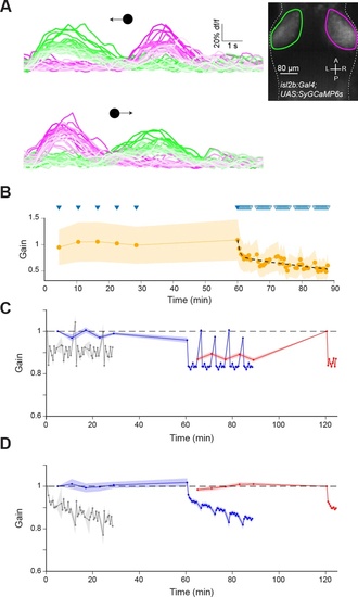
(A) Calcium imaging of RGC axon terminals in OT in an isl2b:GAL4;UAS:SyGC6s transgenic larva during leftward (top) and rightward (bottom) moving spot stimuli. Faint lines indicate later presentations. Inset: Mean z-projection of an image volume showing the left (green) and right (magenta) ROIs containing RGC axon terminals in the tectum. (B) RGC axon terminal responses (n=4 fish) normalised by the mean of the first two responses in each fish. Triangles indicate stimulus presentation times, filled triangles indicate epochs used to establish the ‘baseline’ response. Data from left and right OT were averaged. (C) Model prediction as per Figure 6, but without implementing RGC adaptation. (D) The net effect of simulated RGC adaptation, computed by taking the difference between the model prediction with and without RGC adaptation. Shaded areas indicate SEM.

Prey-catching behavior is modulated by tectal network state and stimulus history.

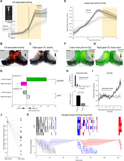
(A) Activity of neurons in the anterior (black) and posterior (grey) OT, triggered on spontaneous CSs. Mean with shaded areas indicating SEM (n=11 fish), dashed line indicates CS time. Inset: Eye tracking and an example of a detected convergent saccade. (B) Mean baseline-subtracted activity of OT cells during 1 s windows centred on spontaneous CSs (orange rectangle in (A), n=66 CSs in a single fish). (C) Baseline-subtracted activity for a single spontaneous CS with rightward post-saccade gaze angle. (D) Comparisons of activity between OT hemispheres for lateralized CSs with leftward (green) and rightward (magenta) post-saccade gaze angle. Error bars indicate SEM (n=408 CSs from 11 fish). (E) Linear drive in the anterior (black) and posterior (grey) OT, prior to CSs, estimated using optimized model parameters and 60 seconds of pre-saccade ongoing activity. Mean with shaded area indicating SEM (n=11 fish). Dashed line indicates baseline linear drive. (F) Linear drive of OT cells during the 10 s prior to spontaneous CSs (orange rectangle in (E), in the same fish depicted in (B), n=66 CSs). (G) Linear drive prior to the spontaneous CS shown in (C). (H) Top: Distribution of r² values for linear fits of CS-associated activity as a function of estimated linear drive (with a positive slope constraint). Linear drive (‘excitability’) of individual neurons was estimated using optimized model parameters and 60 s of pre-saccade ongoing activity (black) or randomly chosen sequences of ongoing activity (grey). 680 CSs from 11 fish. Bottom: median r² values, error bars indicate ±1%, p-values for a Wilcoxon signed rank test. (I) For each of the CSs, the mean across neurons of CS-associated activity was computed for bins of estimated linear drive. Shaded area indicates bin-wise SEM. (J) Rate of spontaneous CSs during rest blocks (more than 120 s since the last visual stimulus presentation) vs visual stimulation blocks, normalised by rest block rate. Each line indicates one fish. (K) Prey-catching responses evoked by very low (grey), high (blue), and low (red) elevation stimuli, presented according to the protocol described in Figure 6. Top raster show responses from each of six animals (rows) and lower trace shows mean response probability with 90% confidence interval.