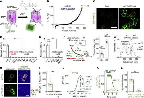
Figure 1. Design, optimization, and characterization of a genetically encoded GRAB_ATP sensor

(A) Schematic drawing depicting the principle of GRAB-based ATP sensors designed using the human P2Y₁ receptor as the scaffold coupled to the circularly permuted enhanced GFP (cpEGFP). Binding of ATP induces a conformational change that increases the fluorescence signal.

(B) Optimization of the N- and C-terminal linkers connecting the hP2Y₁ receptor and the cpEGFP moiety, yielding increasingly responsive ATP sensors. The sensor with the highest response to 100 μM ATP, GRAB_ATP1.0 (ATP1.0), is indicated.

(C) Representative fluorescence images of HEK293T cells expressing the ATP1.0 sensor under the basal condition and in the presence of 100 μM ATP.

(D and E) Summary of ΔF/F₀ measured in ATP1.0-expressing HEK293T cells in the presence of the indicated compounds (each at 10 μM, except for MRS-2500, which was applied at 30 μM), normalized to the peak response measured in ATP; n = 4 independent wells each. ATP, adenosine triphosphate; MRS, MRS-2500; Glu, glutamate; GABA, γ-aminobutyric acid; Gly, glycine; DA, dopamine; NE, norepinephrine; 5-HT, 5-hydroxytryptamine (serotonin); HA, histamine; ACh, acetylcholine; ADP, adenosine diphosphate; AMP, adenosine monophosphate; Ado, adenosine; UDP, uridine diphosphate; UDP-G, UDP-glucose.

(F) Summary of the response kinetics of ATP1.0. Left: the experimental system and representative fluorescence traces of ATP1.0 and co-expressed mCherry-CAAX in HEK293T cell to locally puffed ATP; a line scan was used to measure the fluorescence response, and ATP was puffed with a glass pipette with the duration of ∼0.5 s (see STAR Methods for details). Right: the time constant of on and off kinetics of ATP1.0; n = 22 cells from seven coverslips.

(G) Excitation (Ex) and emission (Em) spectra of the ATP1.0 sensor in the presence of ATP (100 μM) or ATP (100 μM) together with MRS-2500 (300 μM). The isosbestic point at 435 nm is indicated.

(H and I) GFP fluorescence images (left column) and pseudocolor images of the response (right column) measured in HEK293T cells expressing ATP1.0 (top row) or pm-iATPSnFR1.0 (bottom row). (I) shows a summary of the response to 100 μM ATP; n = 40 and n = 30 cells each for ATP1.0 and pm-iATPSnFR1.0, respectively.

(J) The peak fluorescence response measured in HEK293T cells expressing ATP1.0 or pm-iATPSnFR1.0 plotted against the indicated concentrations of ATP; n = 10 and n = 20 cells each, respectively. Inset: the same data, normalized and re-plotted.

(K and L) The fluorescence response (K) and signal-to-noise ratio (L) measured in HEK293T cells expressing ATP1.0 or the FRET-based ecAT3.10 sensor; where indicated, 100 μM ATP was applied; n = 20 cells each. The signal-to-noise ratio is defined as the peak response divided by the SD prior to the application of ATP application.

Scale bars represent 30 μm. Summary data are presented as mean ± SEM. The data in (D) and (E) were analyzed using one-way ANOVA followed by Dunnett’s post hoc test; the data in (I) and (L) were analyzed using Student’s t test; ^∗∗∗p < 0.001; n.s., not significant (p > 0.05). See also Figures S1, S2, and S6.

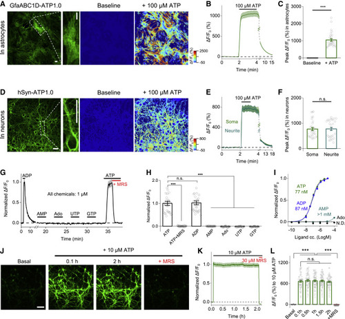
Figure 2. Characterization of the GRAB_ATP1.0 sensor in primary cultured astrocytes and neurons

(A–C) ATP1.0 was expressed in cultured cortical astrocytes and measured using confocal imaging. (A) Raw GFP fluorescence image (left) and pseudocolor images of the baseline and peak response (ΔF/F₀) to 100 μM ATP. (B) Time course of ΔF/F₀; 100 μM ATP was applied where indicated. (C) Summary of the peak ΔF/F₀ measured before and after application of 100 μM ATP; n = 30 regions of interest (ROIs) each from three coverslips.

(D–F) Same as (A)–(C), except ATP1.0 was expressed in cultured rat cortical neurons; n = 30 ROIs each from three coverslips.

(G–I) Normalized ΔF/F₀ measured in cultured neurons expressing ATP1.0, showing an example trace (G), summary data (H), and dose-response curves with corresponding EC₅₀ values (I). UTP, uridine triphosphate; GTP, guanosine triphosphate; N.D., not determined. n = 30–91 ROIs from three coverslips (H and I).

(J–L) Fluorescence image (J), trace (K), and summary (L) of ATP1.0 expressed in cultured hippocampal neurons during a 2 h application of 10 μM ATP; n = 60 neurons from three coverslips.

Scale bars represent 30 μm (A and D) and 100 μm (J). Summary data are presented as mean ± SEM. The data in (C) and (F) were analyzed using Student’s t test; the data in (H) and (L) were analyzed using one-way ANOVA followed by Bonferroni’s multiple-comparison test; ^∗∗∗p < 0.001; n.s., not significant. See also Figures S3 and S6.

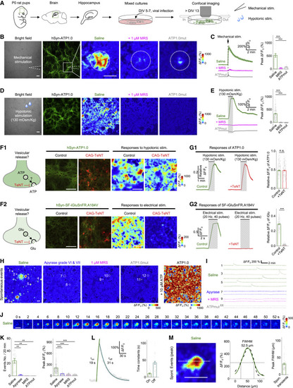
Figure 3. GRAB_ATP1.0 can be used to detect ATP release in primary hippocampal cultures

(A) Schematic diagram depicting the experimental protocol in which primary hippocampal neurons are cultured and infected with an AAV encoding ATP1.0 or ATP1.0mut under the control of the hSyn promoter, followed by confocal fluorescence microscopy during various stimuli. DIV, days in vitro.

(B–E) Bright-field images, GFP fluorescence images, pseudocolor images (B and D), and average traces (C and E, left) of the fluorescence response of ATP1.0 or ATP1.0mut measured in saline or 1 μM MRS-2500 (MRS). The white dashed circles in (B) indicate the 150-μm-diameter ROI used for analysis, and the white dashed lines in (B) indicate the location of the electrode used for mechanical stimulation. The summary data (C and E, right) represent 13–20 ROIs from three coverslips (C) and 168–214 ROIs from three or four coverslips (E).

(F1 and G1) Fluorescence images of ATP1.0 (green) and EBFP2-iP2A-TeNT (red) (F1), pseudocolor images (F1), average traces (G1, left), and summary data (G1, right); n = 217–227 ROIs from four coverslips each.

(F2 and G2) Fluorescence images of SF-iGluSnFR.A184V (green) and TeNT-BFP2 (red) (F2), pseudocolor images (F2), average traces (G2, left panels), and summary data (G2, right); n = 171 ROIs from three coverslips each.

(H) Cumulative transient change in ATP1.0 or ATP1.0mut fluorescence measured during 20 min of recording in saline, apyrase (15 U/mL VI plus 15 U/mL VII), or 1 μM MRS-2500. The white dashed circles indicate the ROIs used for the analyses in (I).

(I) Representative traces of ΔF/F₀ measured under the indicated conditions.

(J) Representative time-lapse pseudocolor images captured in saline.

(K) Quantification of the number of events per 20 min (left) and the peak fluorescence response (right) in neurons expressing ATP1.0 or ATP1.0mut; n = 114–363 ROIs from three to ten coverslips.

(L and M) Kinetics profile (L) and spatial profile (M) of the change in ATP1.0 fluorescence measured in saline. The summary in (L) and (M) data represent 54 events and 128 events, respectively, from four coverslips. FWHM, full width at half maximum.

Scale bars represent 100 μm. Summary data are presented as the mean ± SEM. The data in (C) and (E) were analyzed using one-way ANOVA followed by Dunnett’s post hoc test; the data in (G) were analyzed using Student’s t test; the data in (K) were analyzed using one-way ANOVA followed by Bonferroni’s multiple-comparison test. ^∗∗p < 0.01 and ^∗∗∗p < 0.001; n.s., not significant. See also Figure S7.

Figure 4. GRAB_ATP1.0 reveals in vivo ATP release induced by injury in a zebrafish model

(A and B) Schematic diagram depicting in vivo confocal imaging of fluorescence changes induced by a localized puff (via a micropipette; see inset) of various compounds in the optic tectum of zebrafish larvae expressing ATP1.0 (Elavl3:Tet^off-ATP1.0) or ATP1.0mut (Elavl3:Tet^off-ATP1.0mut).

(C) Representative fluorescence images (left), traces (middle), and summary (right) showing the response of ATP1.0 or ATP1.0mut to the indicated compounds. Arrows indicate the localized application of saline (Control) or ATP (5 mM). Where indicated, MRS-2500 (90 μM) was applied; n = 6 or 7 fishes.

(D) Schematic diagram depicting confocal imaging of ATP1.0 responses before and after two-photon laser ablation (i.e., injury) in the optic tectum of zebrafish larvae expressing ATP1.0. The red dashed circle indicates the region of laser ablation, and the black dashed rectangle indicates the imaging region shown in (E).

(E) Time-lapse pseudocolor images showing the response of ATP1.0 to laser ablation in the optic tectum. The laser ablation was performed at time 0 s and lasted for 7 s, and the ATP1.0 fluorescence was imaged beginning 2 min before laser ablation.

(F) Schematic diagram showing dual-color confocal imaging of ATP release and microglial migration before and after laser ablation in transgenic zebrafish Tg(coro1a:DsRed) larvae expressing ATP1.0. In Tg(coro1a:DsRed) larvae, the microglia express DsRed. The red dashed circle indicates the region of laser ablation, and the black dashed rectangle indicates imaging region.

(G) In vivo time-lapse confocal images showing the migration of microglia (red) and the change in ATP1.0 fluorescence (green) before and after laser ablation (start at time 0 s). The green dashed circle indicates the boundary of the ATP wave at 300 s, and the signal measured in the green dashed circle was used for the analysis in (J). Green arrows indicate the protrusions of microglia entering the green dashed circle; solid yellow arrows indicate the cell bodies of microglia entering the green dashed circle.

(H) Summary of the ATP1.0 response in different distances to the injury site, measured at 0, 11, 21, and 300 s after injury.

(I) Time course of the ATP1.0 response measured at 15 and 30 μm from the site of laser ablation. The arrow shown in traces indicates the beginning of the 7 s laser ablation.

(J) Time course of the ATP1.0 response (green) and the microglia migration (red) before and after laser ablation (vertical arrow); also shown is a trace of DsRed fluorescence measured in the area without laser ablation of the same larvae. ROIs 60 μm in diameter are used for analysis.

Scale bars represent 40 μm (B) and (C), 100 μm (E), and 30 μm (G). Data shown in (C) and (J) are presented as mean ± SEM; data shown in (H) and (I) are presented as mean + SEM; numbers in parentheses in (H)–(J) represent the number of zebrafish larvae in each group. The data in (C) were analyzed using Student’s t test; ^∗∗∗p < 0.001. See also Figures S4 and S7 and Video S1.

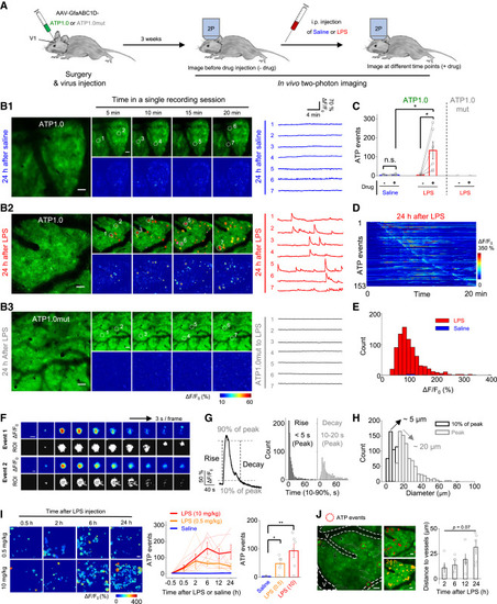
Figure 5. GRAB_ATP1.0 reveals localized ATP-release events in mouse brain following LPS-induced systemic inflammation

(A) Schematic diagram depicting the experimental protocol in which an AAV encoding either ATP1.0 or ATP1.0mut under the control of the GfaABC1D promoter is injected into the mouse visual cortex (V1), followed by two-photon imaging (2P) through a cranial window at various times after an intraperitoneal (i.p.) injection of saline or lipopolysaccharides (LPS).

(B1 and B2) Representative fluorescence images, pseudocolor images, and individual traces of the fluorescence response of ATP1.0 measured 24 h after saline (B1) or 10 mg/kg LPS (B2) injection. Indicated regions of interest (ROIs, white dashed circles) are identified using AQuA software overlay.

(B3) Same as (B2), except the ATP1.0mut sensor is expressed.

(C) Summary of the number of localized ATP events measured during a 20 min recording before (−) and after (+) saline or 10 mg/kg LPS injection; n = 5 or 6 mice each.

(D) Pseudocolor images showing all the identified ATP events in an exemplar ATP1.0-expressing mice after 24 h LPS injection. The number of identified ATP events from one mouse is shown on the y axis.

(E) Distribution of the peak fluorescence response (ΔF/F₀) of the localized ATP events measured in ATP1.0-expressing mice 24 h after 10 mg/kg LPS (red) or saline (blue) injection; n = 805 events from six mice and 25 events from five mice, respectively.

(F) Detailed analysis of the properties of two individual localized ATP events shown as pseudocolor images of ΔF/F₀ and the corresponding ROIs identified using AQuA software at 3 s intervals.

(G) Left: a representative trace (averaged from 50 peak-aligned events) showing the rise and decay kinetics of the event, defined the time between 10% and 90% of the baseline to peak. Right: summary of rise and decay times; n = 805 events from six mice.

(H) Distribution of the size of individual events at 10% of peak response (black) and peak response (gray) measured in ATP1.0-expressing mice 24 h after 10 mg/kg LPS injection; n = 805 events from six mice.

(I) Left: representative images showing ATP-release events (indicated as ROIs) in ATP1.0-expressing mice at the indicated times after 0.5 and 10 mg/kg LPS injection. Middle and right: summary of the number of ATP-release events after 0.5 mg/kg LPS, 10 mg/kg LPS, or saline injection. The data from each individual mouse and the average data are shown. n = 6, n = 6, and n = 5 mice for the 0.5 mg/kg LPS, 10 mg/kg LPS, and saline groups, respectively.

(J) Left: representative image showing early ATP-release events red dashed circles) located near the blood vessel (V, indicated by white dashed lines). Middle, images taken 2 h (red) and 24 h (yellow) after 10 mg/kg LPS injection. Right: summary of the distance between the events and the blood vessel at the indicated times after 10 mg/kg LPS injection; n = 5 mice.

Scale bars represent 50 μm (B, I, and J) and 5 μm (F). Summary data are presented as mean ± SEM. The data in (C) were analyzed using Student’s t test; the data in (J) were analyzed using one-way ANOVA followed by Dunnett’s post hoc test; ^∗p < 0.05; ^∗∗p < 0.01; n.s., not significant. See also Figure S5 and Video S2.