a Schematic diagram of the closed-loop virtual reality setup. Four displays presented visual stimuli. Tail beating was captured by a camera and caused the scenery to move backward to create the impression of forward swimming. The virtual traveling distance was calculated by [frequency of tail beats] × [gain]. b Schematic drawing of the tethered adult zebrafish using a custom-made harness, dental bond, and cement. Two needle electrodes were placed on both sides of the body to deliver electric shocks. c The imaged region in the telencephalon. The side (top) and dorsal (bottom left) views and coronal section (bottom right) of the adult zebrafish brain. The blue box indicates the imaged region by surface three-plane imaging, and the red box indicates the additionally imaged region by six-plane imaging. Dc, central zone of dorsal telencephalic area; Dl, lateral zone of dorsal telencephalic area; Dm, medial zone of dorsal telencephalic area; OB, olfactory bulb; OT, optic tectum; Sy, sulcus ypsiloniformis; Tel, telencephalon. d Calcium imaging of neural activity in three focal planes using the piezo actuator. Either left or right hemisphere was imaged. These images are averaged images of the left hemisphere in three focal planes. Anterior to top; lateral to left; medial to right. Dl, lateral zone of the dorsal telencephalon; Dc, central zone of dorsal telencephalon; Dm, medial zone of dorsal telencephalon¹⁰. e Schema of alternate switching of neural activity detection by a two-photon microscope and visual stimulation by displays. Green arrows indicate the duration of scanning; in this setting, the detector is ON and displays are OFF. Blue arrows indicate the duration from the end of a line scan to the onset of the next line scan; in this setting, the detector is OFF and displays are ON.

a GO/NOGO tasks in the virtual reality system. b The learning curve of GO/NOGO trials of a fish that met the behavioral learning criterion. Horizontal dotted line, the criterion for behavioral learning; open circles, successful trials; solid circles, failed trials; vertical line, the initiation time point of trials with electric shock; vertical dotted line, the initiation of the next session. c Left: the number of trials needed until the behavioral learning criterion of GO and NOGO trials was satisfied in the Xth session and the next X + 1th session (32 fish). Xth GO vs X + 1th GO, ^***P = 7.72 × 10⁻⁶; Xth NOGO vs X + 1th NOGO, ^**P = 4.03 × 10⁻³. Two-tailed paired t-test. Right: Comparison of the success rates among control, unpaired, and learner groups at the 22nd GO trial and16th NOGO trial which were the average numbers needed to achieve the behavior criteria in standard learner fish. Control (w/o shock) vs learner, ^***P = 7.52 × 10⁻⁸; unpaired vs learner, ^***P = 2.27 × 10⁻⁶, two-tailed unpaired t-test. Columns and error bars: mean ± SEM. Each circle represents one fish. The numbers in parentheses are the number of fish used in the statistics. d Imaging data analysis procedure. See “Methods” for details. e Similarity to GO and NOGO templates in the adaptation stage (upper panel), initial stage of training (bottom left panel), and after the establishment of behavioral learning (bottom right panel). Horizontal bars in the upper and lower positions indicate the period of GO and NOGO trials, respectively. The bar colors indicate the color of the environment at the position of the fish. f Enlarged view of the boxed area in (e, bottom right panel). g Comparison of peak value of the similarities to both GO and NOGO templates in both trials in the adaptation stage, after behavioral learning, and after reaching the goal after behavioral learning. Columns and error bars: mean ± SEM. Circles in the adaptation stage and after behavioral learning indicate peak similarities when the fish was in the start color in the first five trials. Circles after reaching the goal indicate peak similarities after fish reached the goal in the first five GO trials after behavioral learning. Adaptation vs after behavioral learning in GO trials GO template, ^**P = 1.56 × 10⁻³; after behavioral learning vs after reaching the goal in GO trials GO template, ^***P = 4.5 × 10⁻⁴; after behavioral learning vs after reaching the goal in GO trials NOGO template, ^***P = 5.02 × 10⁻⁵; adaptation vs after behavioral learning in NOGO trials NOGO template, ^***P = 1.56 × 10⁻⁶. Two-tailed unpaired t-test.

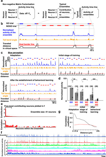
a The formula to calculate the non-negative matrix factorization (NMF; for details, see “Methods”). b The activity of the blue perception-coding ensemble as an example of an activity pattern (the activity in this panel is a part of c, bottom left panel). The blue line indicates the activity of a neural ensemble normalized by the self-maximum value. The horizontal bars in the upper and lower positions indicate the period of GO and NOGO trials, respectively. The bar colors indicate the color of the environment at the position of the fish. Orange line, the tail bend angle. Black line, the distance that fish had traveled. Red line, the point of color change. c The activity of the blue perception-coding ensemble in the adaptation stage (upper left panel), initial stage of training (upper right panel), and after behavioral learning was established (bottom left panel). d Quantified activity of the blue perception-coding ensemble in the adaptation stage, initial stage of training, and after behavioral learning was established. Columns and error bars: mean ± SEM. Circles indicate the peak value in each GO or NOGO trial. The numbers in parentheses are the number of trials used in the statistics. Adaptation GO vs adaptation NOGO, ^**P = 3.06 × 10⁻³; initial stage of training GO vs initial stage of training NOGO, ^***P = 1.67 × 10⁻⁵; after behavioral learning GO vs after behavioral learning NOGO, ^***P = 1.96 × 10⁻⁶, F(5, 92) = 26.25. One-way ANOVA, Bonferroni’s multiple comparison test. e Contribution of each neuron within the ensemble (upper panel) and correlation coefficient of each neuron’s activity to the ensemble’s activity (lower panel). f The activity of the ensemble (top trace) and the five most-contributing neurons in the ensemble (descending order from the top). Dotted lines indicate the timing when the neurons showed simultaneous activation with the ensemble. g Relationship between the correlation coefficient and distance for the 10 most-contributing neurons in the ensemble encoding the perception of blue. The data were averaged from 27 fish with this ensemble. Black line denotes the averaged correlation from 27 fish. Red line denotes the average of averaged 10 shuffled data from 27 fish (see “Methods”).

Notations in the figures are all the same as in Fig.3b. a The activity of two neural ensembles (cyan and magenta lines) in the adaptation stage (left panel) and the stages immediately before (middle panel) and after (right panel) behavioral learning was established. b Enlarged view of the activity of the two ensembles in the boxed area in (a). The vertical gray line indicates the time point when the fish reached the goal. c Comparison of the cyan ensemble’s peak activity in the GO trials in different learning stages. Columns and error bars: mean ± SEM. Each circle indicates the value in each GO trial. The number in parentheses is the number of trials used in the statistics. Adaptation vs immediately before behavioral learning, ^***P = 2.60 × 10⁻¹⁶; adaptation vs after behavioral learning, ^***P = 6.43 × 10⁻¹³, F(3, 55) = 82.85. One-way ANOVA, Bonferroni’s multiple comparison test. d Comparison of the magenta ensemble’s peak activity when fish perceived red color in GO and NOGO trials in different learning stages. Columns and error bars: mean ± SEM. Each circle indicates the value in each trial. The numbers in parentheses are the number of trials used in the statistics. Red GO before behavioral learning vs Red GO after behavioral learning, ^**P = 7.91 × 10⁻³; red NOGO before behavioral learning vs red NOGO after behavioral learning, ^**P = 6.48 × 10⁻³, F(7, 80) = 9.25. One-way ANOVA, Bonferroni’s multiple comparison test. e–h Results of the same analysis as (a–d) above for another fish. g The numbers in parentheses are the number of trials used in the statistics. Adaptation vs immediately before behavioral learning, ^**P = 1.94 × 10⁻³; adaptation vs after behavioral learning, ^***P = 2.44 × 10⁻⁵, F(3, 56) = 13.02 One-way ANOVA, Bonferroni’s multiple comparison test. h The numbers in parentheses are the number of trials used in the statistics. Red GO adaptation vs red GO intermediate stage, P = 0.295; red NOGO adaptation vs red NOGO intermediate stage, ^***P = 9.085 × 10⁻¹¹, F(7, 88) = 31.67. One-way ANOVA, Bonferroni’s multiple comparison test. Red GO adaptation vs red GO intermediate stage, ^**P = 1.42 × 10⁻³. Two-tailed unpaired t-test. i Relationship between the correlation coefficient and distance among the 10 most-contributing neurons in the color rule-encoding ensembles (left, blue is dangerous rule; right, red is safe rule). The data were averaged from the fish with these ensembles. Black line denotes the averaged correlation from all fish. Red line denotes the average of averaged 10 shuffled data from the fish (see “Methods”).

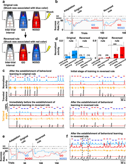
a GO/NOGO tasks with the original and reversed rules. b The learning curve of GO/NOGO trials with the original and reversed rules. Vertical line, initiation of the original rule; vertical dotted line, initiation of the reversed rule. In the adaptation and with the original rule, the success rates of GO and NOGO trials are indicated by blue and red lines, respectively. In the reversed rule, the success rates of GO and NOGO trials are indicated by red and blue lines, respectively. Open circle indicates successful trial. Solid circle indicates failed trial. c The activity of two ensembles after behavioral learning was established with the original rule (upper left panel), immediately after rule change (upper right panel), and immediately before (bottom left panel) and after (bottom right panel) behavioral learning was established with the reversed rule. d Left: comparison of the cyan ensemble’s peak activity in (c) when fish perceived blue color as a starting color with the original and reversed rules in the initial stage of training and after behavioral learning. Columns and error bars: mean ± SEM. Each circle indicates the value in each trial. After behavioral learning of original rule vs after behavioral learning of reversed rule, ^***P = 1.80 × 10⁻⁶, F(3, 75) = 14.28. One-way ANOVA, Bonferroni’s multiple comparison test. Right: comparison of the red ensemble’s peak activity in (c) when fish perceived red color as a starting color with the original and reversed rules in the initial stage of training and after behavioral learning. Columns and error bars: mean ± SEM. Each circle indicates the value in each trial. The numbers in parentheses are the number of trials used in the statistics. After behavioral learning of original rule vs after behavioral learning of reversed rule, ^***P = 9.73 × 10⁻¹⁰, F(3, 36) = 36.34. One-way ANOVA, Bonferroni’s multiple comparison test. e The learning curve of GO/NOGO trials of another fish in which the cyan ensemble did not disappear. Notations are identical to (b). f The activity of the two ensembles after behavioral learning was established with the reversed rule. The cyan and red lines indicate the ensembles encoding the color rule that blue is dangerous and red is dangerous, respectively.

Notations in the figures are identical to Fig 3b. a The open-loop experiment in which feedback was turned off. The scenery did not move in response to the tail beat. b, c The activity of the two ensembles encoding the color rules that blue is dangerous (cyan line) and that red is safe (magenta line) in the open-loop condition. b Data from the fish used in Fig.4a–d. c Data from the fish used in Fig.4e–h. d The activity of an ensemble in the open-loop condition (upper left panel), after behavioral learning was established (upper right panel), in the adaptation (middle left panel), and in the initial stage of training (bottom left panel). The activity of the ensemble increased in the GO trial in the open-loop condition and the failed GO trial but not in the successful GO trials in the closed-loop condition. e Left: enlarged view of a failed GO trial (boxed area of the dotted line in (d) upper right panel). Right: enlarged view of a successful GO trial (boxed area of the dashed line in (d) upper right panel). Red rectangle indicates the timing of shock. f Comparison of peak activity of the ensemble when fish perceived the starting color in the adaptation stage, initial stage of training, successful GO trials, failed GO trials, and open-loop GO trials. Columns and error bars: mean ± SEM. Each circle indicates the value in each GO trial. The numbers in parentheses are the number of trials used in the statistics. Successful GO vs failed GO, ^***P = 7.79 × 10⁻¹³; successful GO vs open-loop, ^***P = 2.54 × 10⁻³⁴, F(4, 110) = 101.97. One-way ANOVA, Bonferroni’s multiple comparison test. g–i Results of the same analysis as (d–f) above for another fish. The timing of the increased activity along with behavioral learning was different from the data shown in (d–f). i The numbers in parentheses are the number of trials used in the statistics. Successful GO vs failed GO, ^***P = 5.02 × 10⁻⁴; successful GO vs open-loop, ^***P = 8.93 × 10⁻⁶, F(4, 53) = 23.86. One-way ANOVA, Bonferroni’s multiple comparison test. j Relationship between the correlation coefficient and distance among the 10 most-contributing neurons in the putatively SFPE-encoding ensemble. The data were averaged from 9 fish with this ensemble. Black line denotes the averaged correlation from 9 fish. Red line denotes the average of averaged 10 shuffled data from 9 fish (see “Methods”).

a, b The traveled distance in five successful GO trials after the establishment of behavioral learning in a fish with both ensembles encoding the color rule that blue is dangerous and the scenery flow prediction error (a) and a fish with only the ensemble encoding the color rule that blue is dangerous (b). The black line indicates the traveled distance. The red line indicates the goal. c Comparison of the period of halts (left panel), number of halts (middle panel), and period of movement (right panel) between two groups. The number of fish which has color rule-coding and putative SFPE ensembles is 8 and that of fish which has only color rule-coding ensemble is 16. Columns and error bars: mean ± SEM. Each circle indicates the value in each fish. Left: ^*P = 0.028 (Cohen’s d = 0.978302). Middle: P = 0.455. Right: P = 0.457. One-tailed unpaired t-test, n.s., not significant.

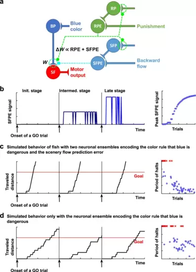
a Schematic circuit diagram to select swimming forward. The neural network comprises ensembles encoding the perception of blue (BP, blue) and swimming forward (SF, red). Moreover, two additional units represent mutually different prediction errors. The reward prediction error (RPE, green) ensemble computes the difference between the (negative) reward prediction (RP) and actual punishment. Whereas, the scenery flow prediction error (SFPE, cyan) computes the difference between the scenery flow prediction (SFP) and actual backward flow. Here, the RPE ensemble took a positive value when the fish could avoid the punishment contrary to its expectation; otherwise, it took zero. The SFPE ensemble self-organized in the early stage of training to take a positive value when the fish sensed the SFPE at a given time point or take zero otherwise. The synaptic potentiation of 𝑊

a, b The traveled distance in five successful GO trials after the establishment of behavioral learning in a fish with both ensembles encoding the color rule that blue is dangerous and the scenery flow prediction error (a) and a fish with only the ensemble encoding the color rule that blue is dangerous (b). The black line indicates the traveled distance. The red line indicates the goal. c Comparison of the period of halts (left panel), number of halts (middle panel), and period of movement (right panel) between two groups. The number of fish which has color rule-coding and putative SFPE ensembles is 8 and that of fish which has only color rule-coding ensemble is 16. Columns and error bars: mean ± SEM. Each circle indicates the value in each fish. Left: ^*P = 0.028 (Cohen’s d = 0.978302). Middle: P = 0.455. Right: P = 0.457. One-tailed unpaired t-test, n.s., not significant.