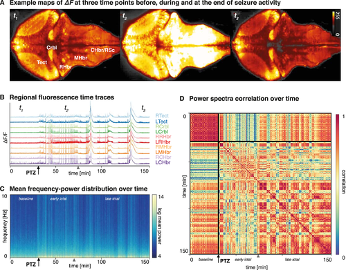
PTZ-iduced seizures recorded in the zebrafish larvae using light sheet imaging.

(A) This image shows heat maps of fluorescence in a single slice of the intact larval zebrafish brain in the xy plane at different time points during the experiment (time points also indicated in Fig 2B). Seizure activity (t₂) is visually apparent as an overall increase in neuronal activity compared to baseline state (t₁). (B) Regionally averaged time traces of the fluorescence signal across 5 bilateral anatomically defined regions are shown for the whole duration of the experiment in a single animal (150 minutes). Seizures are readily apparent as an inrease in generalised and apparently synchronous high amplitude activity. (C) Average Fourier power spectra across fish and across all brain regions are plotted against time for the duration of the experiment, using a sliding window estimator (length: 60s, step: 10s), with colours indicating log-power. The graph is a the average over n = 3 fish. PTZ causes an increase largely in low frequencies (<2Hz), with intermittent bursts of more broadband activity. (D) A correlation matrix showing correlation indices of the power-distribution patterns across different time points (delay-delay matrix). This reveals three distinct time periods, corresponding to baseline (<30min), ictal (30-70min) and late ictal (>70min) phases with distinct spectral signatures and temporal dynamics. Tect—Tectum, Crbl—Cerebellum, RHbr—Rostral Hindbrain, MHbr—Mid-Hindbrain, CHbr/RSc—Caudal Hindbrain/Rostral Spinal Cord.

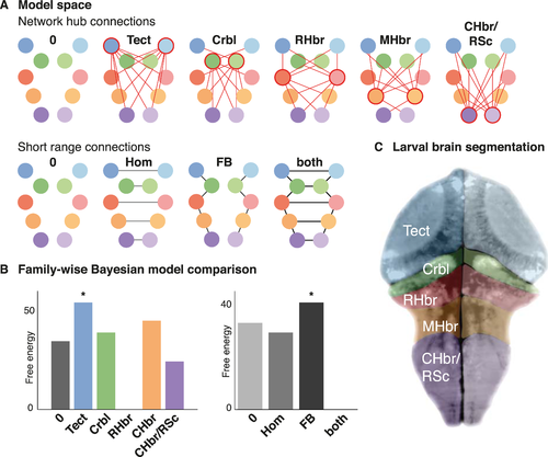
Network model architecture during interictal background activity.

(A) Two aspects of a factorial model space are shown: extrinsic connectivity of putative network hubs (yielding 6 types of models), and short range connection between neighbouring and homotopic nodes (yielding 4 different types of models); a total of 6 * 4 = 24 models were evaluated, where any one model is combines one of the network hub connectivity architectures with a short-range connectivity setup. Bayesian model reduction was used to estimate the model evidence across this model space characterised by the presence or absence of these defined sets of between-region reciprocal connections (neighbouring, homotopic, and hub connections). (B) For each model family (corresponding to the factorial model space), the free energy difference to the worst-performing model is shown. In DCM, the free energy difference is used to approximate model log-likelihood differences: Asterisks indicate the winning model family identified from Bayesian model selection. These results indicate that the model with neighbouring, and homotopic connections as well as the optic tectum with hub-like connectivity best explain the observed spontaneous activity at baseline. (C) Mapping of the ROIs for this analysis is illustrated as overlay on a single fluorescence image taken from one of the animals included in this study. Areas were identified based on visible neuroanatomical landmarks and correspond to the nodes of the same colour in the network representations of the model space.

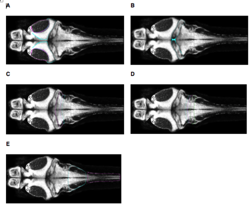
Atlas regions corresponding to the anatomical segmentation used in our analysis (all images at z = -90.

(A) ‘Tectum’ corresponds to Z Brain regions Tectum Stratum Periventriculare and Tectum Neuropil. (B) ‘Cerebellum’ corresponds to Z Brain region Cerebellum. (C) ‘Rostral Hindbrain’ corresponds to Z Brain regions Rhombomere 2 and Rhombomere 3. (D) ‘Mid Hindbrain’ corresponds to Z Brain region Rhombomere 4, Rhombomere 5, and Rhombomere 6. (E) ‘Caudal Hindbrain / Rostral Spinal Cord’ corresponds to Z Brain regions Rhombomere 7, and Spinal Cord. Images are taken from https://engertlab.fas.harvard.edu/Z-Brain [accessed 18/05/2018].