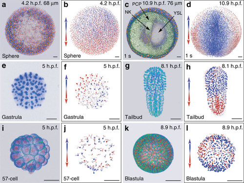
Reconstructing early embryogenesis from time-lapse optical sectioning.

(a-d) Danio rerio data set Dr1, animal pole (AP) view; (a,b) sphere stage, volume cut at 68 µm of the AP to visualize deep cells; (c,d) 1-somite stage (1 s), volume cut at 76 µm of the AP; NK, neural keel; PCP, prechordal plate; YSL, yolk syncytial layer. (e-h) Phallusia mammillata data set Pm1, vegetal view, circum notochord side up; (e,f) gastrula stage; (g,h) tailbud stage. (i-l) Paracentrotus lividus data set Pl1, lateral view, AP up; (i,j) 57-cell stage; (k,l) blastula stage. (a,c,e,g,i,k) 3D raw data visualization (with Amira software), hours post fertilization (h.p.f.) indicated top right, developmental stage indicated bottom left, scale bars, 50 µm. (a,c,i,k) Nuclear staining from H2B-mCherry mRNA injection (in orange), membrane staining from eGFP-HRAS mRNA injection (in green). (e,g) Nuclear staining from H2B-eGFP mRNA injection (in blue-green). (b,d,f,h,j,l) Reconstructed embryo visualized with the Mov-IT tool, corresponding to (a,c,e,g,i,k), respectively. Each cell is represented by a dot with a vector showing its path over the next time steps (15 for the zebrafish data, 9 for the ascidian and sea urchin data). Colour code indicates cell displacement orientation.

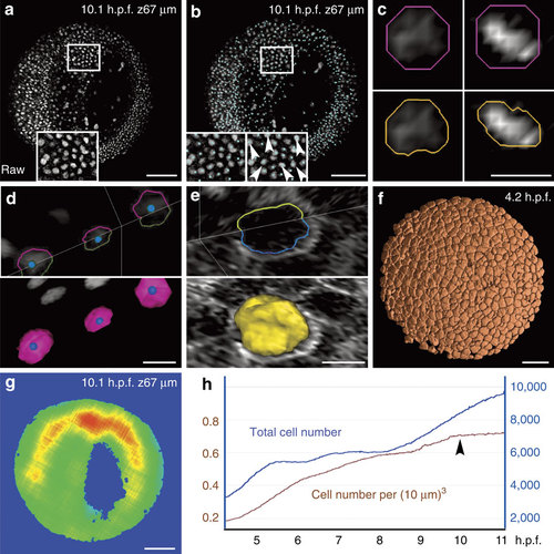
Chain of PDE-based algorithms for the 3D segmentation of embryonic cells.

Results from the zebrafish data set Dr1. Scale bars in µm (100 in a,b,f,g, 10 in c,d,e). (a) Raw data image; single z section at 67 µm depth (orientation as in Fig. 2d), magnification in inset. (b) Nucleus centre detection by the FBLS method, after filtering by GMCF; approximate centres (cyan cubes) superimposed on raw data (grey levels, same orthoslice as a). Magnification in insets: left inset at depth 67 µm; right inset located one section deeper, showing that several centres not displayed at 67 µm were in fact correctly detected and visible below the chosen plane (white arrowheads); remaining centres can be found on other planes using the Mov-IT interactive visualization tool. (c) Nucleus segmentation by SubSurf method; left panels: an interphase nucleus; right panels: a metaphase nucleus; top panels: initial segmentation (pink contour) superimposed on raw data (grey levels); bottom panels: final segmentation (orange contours) superimposed on the same raw data. (d) Nucleus segmentation by SubSurf method; top panel: three nuclear contours superimposed on two raw-data orthoslices; bottom panel: 3D rendering of the segmented nuclei on a single orthoslice. (e) Membrane segmentation by SubSurf method; top panel: one cell membrane contour superimposed on two-raw data orthoslices; bottom panel: 3D rendering of the segmented membrane shape on a single orthoslice. (f) 3D rendering of segmented cell shapes. (g) Embryo shape segmentation; local cell density increasing from blue to red (same orthoslice as a). (h) Total cell number (blue curve) and cell density (brown curve) as a function of time; arrow indicates the end of gastrulation correlating with a plateau in cell density.

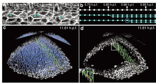
Visualization and validation of the lineage tree reconstruction (zebrafish dataset Dr1).

Results from the zebrafish data set Dr1. All screenshots taken from the Mov-IT visualization interface, then tagged. (a) Cell division illustrated by three snapshots; time in hours post fertilization (h.p.f.) indicated top right; cell centres (cyan cubes) and cell paths (cyan lines) superimposed on two raw-data orthoslices showing the membranes (grey levels). (b) Flat representation of the cell lineage tree for three cell clones over 17 consecutive time steps: each cell is represented by a series of cyan squares, linked according to the cell’s clonal history; the cell dividing in Fig. 4a is circled. (c,d) Nucleus centre detection in a subpopulation of cells chosen at 11.61 h.p.f. Mov-IT visualization in ′checking mode′ adding short vertical white lines to the detected centres, and displaying correct nuclei in green and false positives in red; (c) all detected nuclei; (d) validated nuclei only.

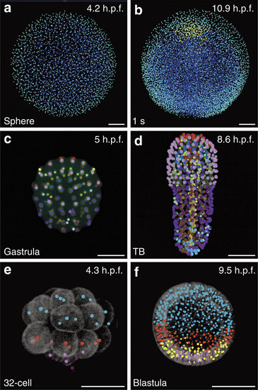
Automated fate map propagation.

Cells were manually selected according to their identity or fate, using the interactive visualization tool Mov-IT. Developmental stages indicated bottom left, developmental times in h.p.f., top right. All scale bars, 50 µm. (a,b) Three cell populations in Danio rerio specimen Dr1, animal pole view; (a) sphere stage, ventral (anterior) up, enveloping layer cells in cyan, epiblast cells in blue; (b) 1-somite stage, same colour code plus hypoblast cells in yellow. (c,d) Fate map in Phallusia mammillata specimen Pm1, vegetal view, circum notochord up, colour code as in ref. 33; (c) gastrula stage; (d) tailbud (TB) stage with automated propagation along the cell lineage of the fate map shown in c. (e,f) Cell populations in Paracentrotus lividus specimen Pl1, lateral view, animal pole up; small micromeres in dark purple, large micromeres in light purple; mesomeres in cyan. (e) 32-cell stage, macromeres in red; (f) blastula stage, Veg1 cell population in red, Veg2 cell population in yellow.