
- Title
-
First steps into the cloud: Using Amazon data storage and computing with Python notebooks
- Authors
- Pollak, D.J., Chawla, G., Andreev, A., Prober, D.A.
- Source
- Full text @ PLoS One
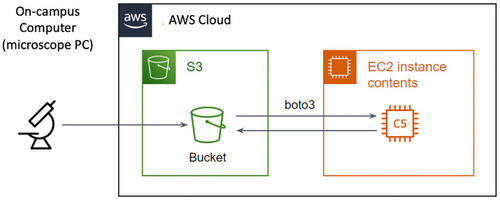
Outline of the pipeline used to work with AWS.
Data from the microscope is moved to S3 data storage using university-provided networks. Data transfer rate can range between 10-100Mb/s. Within AWS cloud infrastructure, data is moved at >10GB/s from storage to EC2 virtual machines to be processed through a Python or Julia Jupyter notebook. |
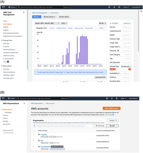
(Top) AWS Organizations portal lists all users and allows addition and creation of new users within the organization. Responsibility for billing of these users are fully on the organization. Creation of new users through Organizations interface is recommended because it allows easy removal of accounts after, for example, student leaves, or the project is finished. (Bottom) Billing Dashboard provides access to multiple tools to manage spending on the level of organization. One of the tools for control is the AWS Cost Management Cost Explorer console. Administrator can check spending by service type (for example, only computing or only storage) and by user account. |
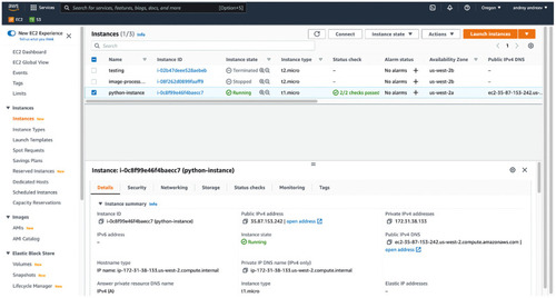
EC2 dashboard showing all launched, stopped, and recently terminated instances.
Running instances are virtual machines, and you are being billed by the second whether you are connected to them or not. Stopped instances are billed for space required to store their memory and data. Stopped instances can be re-started, but state of the memory (RAM) is not guaranteed to be preserved. |
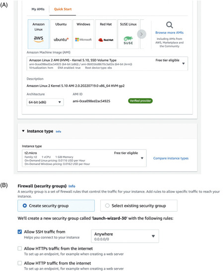
(Right) To launch an EC2 instance, you need to pick an operating system (standard Amazon Linux will provide flexibility for new users) and technical parameters, such as CPU power and memory (RAM). Standard unit of computing power is virtual CPU, vCPU. There is no linear relationship between physical processors and vCPU, but one virtual CPU unit corresponds to a single thread. Correctly selecting the number of vCPUs for your code might require experimenting. Some instances come with graphical processing units (GPU), other instances provide access to fast solid-state drive storage. (Right) Second part of launching an instance is selecting access rules. It includes setting up private-public key pair for passwordless login, and allowing firewall rules for SSH traffic (terminal) and potentially also traffic on ports associated with Jupyter notebook server (such as 8000 port). |
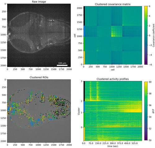
Analysis pipeline for Suite2P-processed data with k-means clustering for k = 4 (four clusters).
Top left: first raw image of the timeseries imaging data. Top right: k-means-clustered covariance matrix of ROIs activity. Color bars on the left correspond to different clusters. Bottom left: Spatial distribution of Suite2P neuron ROIs colored according to covariance matrix clustering. Colors indicate cluster membership according to k-means clustering of the covariance matrix. Bottom right: Activity traces for each Suite2P ROI. Color bars on the left indicate cluster membership according to k-means clustering of the covariance matrix. |