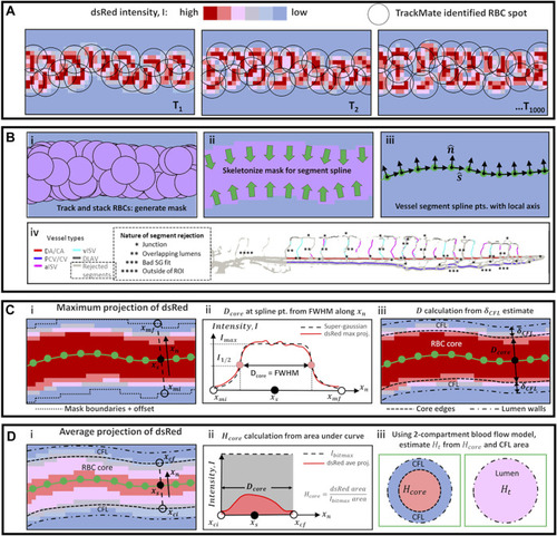
Schematic diagrams of methods used for automated vessel labeling, data filtering, and vessel diameter and hematocrit calculation. (A) High speed image sequence of dsRed intensity was the only collected data from experiments. (B) Series of steps using TrackMate data (i–iii) to obtain vessel spline segment points and directions s^ and n^, and (iv) perform script-automated vessel-type labeling and data filtering from the spline segment skeletons in iii (see text for explanation). (C) Sequence of steps to calculate the width of the RBC core (Dcore) at a spline location (i) by evaluating the full-width-half-maximum (FWHM) range of the Super-gaussian fit to the maximum projection signal (ii). The lumen diameter D is obtained by iterative evaluation (see text) of the cell-free plasma layer (CFL) thickness (δCFL). (D) Sequence of steps to calculate the core hematocrit (Hcore) at a spline location (i) by taking the area fraction between ceiling intensity (Ibitmax) and the average projection signal within the RBC core width (ii). The tube hematocrit in the lumen (Ht) is evaluated by considering the effective contribution of RBC-rich core and plasma-rich CFL.

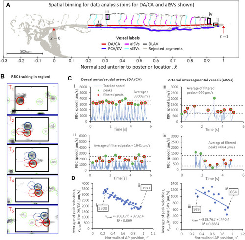
Series of script-automated steps to obtain peak (systolic) RBC velocity from TrackMate data, demonstrated using data from zebrafish 28 of the 2 dpf data set. (A) Velocity sampling within spatial bins of controlled intervals in different vessel types: shown in bold line black boxes are the 60-µm intervals for (i) a region in the anterior DA/CA, (ii) a region in the posterior DA/CA and ventral-to-dorsal intervals of filtered data (see text) for aISVs at the (iii) anterior and (iv) posterior regions of the trunk vasculature. (B) Example of TrackMate particle tracking algorithm performed in the anterior DA/CA region (i) shown in (A). (C) Contiguous velocity against time curves and the application of peak scanning and outlier filtering to obtain the average peak (systolic) velocities in regions i, ii, iii and iv shown in (A). (D) The anterior-to-posterior distribution of average peak velocities in the DA/CA (left) and aISVs (right) with the values for the four locations (i–iv) highlighted in (A,C) shown in boxes.

Spatial distribution map of data in zebrafish 28 of the 2 dpf data set after automated spatial bin averaging: (A) vessel type, (B) average velocity peak (Vpeak), (C) lumen diameter (D), (D) discharge hematocrit (Hd), (E) apparent blood viscosity (η) and (F) average peak WSS (WSSpeak). Arrows in Panels (B–F) indicate the aISV data. See Supplementary Video S13 for maps of hemodynamic quantities for all zebrafish across all the developmental stages analyzed.

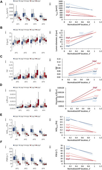
Developmental trends of morphological and hemodynamic quantities in the dorsal aorta/caudal artery (DA/CA). (A) The changes in Vpeak at four regions along the anterior-to-posterior (AP) axis (i) and the AP trend for Vpeak(ii). (B) The changes in D at four AP regions (i) and the AP trend for D(ii). (C) The changes in Hd at four AP regions (i) and the AP trend for Hd(ii). (D) The changes in η at four AP regions (i) and the AP trend for η(ii). (E) The changes in WSSpeak at four AP regions (i) and the AP trend for WSSpeak(ii). (F) The changes in PSR at four AP regions (i) and the AP trend for PSR(ii). Box plots in (i) of Panels (A–D) show the median and the first (Q1) and third (Q3) quartile levels of the hemodynamic quantity for the pooled zebrafish data. The whisker bars represent the maximum and minimum ranges of the data that lie within 1.5 times of the interquartile range (IQR = Q3 − Q1) beyond Q1 and Q3.

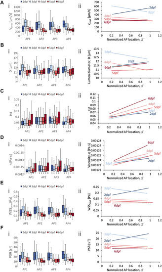
Developmental trends of morphological and hemodynamic quantities in the posterior cardinal vein/caudal vein plexus (PCV/CVP). (A) The changes in Vpeak at four regions along the anterior-to-posterior (AP) axis (i) and the AP trend for Vpeak(ii). (B) The changes in D at four AP regions (i) and the AP trend for D (ii). (C) The changes in Hd at four AP regions (i) and the AP trend for Hd(ii). (D) The changes in η at four AP regions (i) and the AP trend for η(ii). (E) The changes in WSSpeak at four AP regions (i) and the AP trend for WSSpeak(ii). (F) The changes in PSR at four AP regions (i) and the AP trend for PSR(ii). Box plots in (i) of Panels (A–D) show the median and the first (Q1) and third (Q3) quartile levels of the hemodynamic quantity for the pooled zebrafish data. The whisker bars represent the maximum and minimum ranges of the data that lie within 1.5 times of the interquartile range (IQR = Q3 − Q1) beyond Q1 and Q3.

Developmental trends of morphological and hemodynamic quantities in the arterial intersegmental vessels (aISVs). (A) The changes in Vpeak at four regions along the anterior-to-posterior (AP) axis (i) and the AP trend for Vpeak(ii). (B) The changes in D at four AP regions (i) and the AP trend for D(ii). (C) The changes in Hd at four AP regions (i) and the AP trend for Hd(ii). (D) The changes in η at four AP regions (i) and the AP trend for η(ii). (E) The changes in WSSpeak at four AP regions (i) and the AP trend for WSSpeak(ii). (F) The changes in PSR at four AP regions (i) and the AP trend for PSR(ii). Box plots in (i) of Panels (A–D) show the median and the first (Q1) and third (Q3) quartile levels of the hemodynamic quantity for the pooled zebrafish data. The whisker bars represent the maximum and minimum ranges of the data that lie within 1.5 times of the interquartile range (IQR = Q3 − Q1) beyond Q1 and Q3.

Developmental trends of morphological and hemodynamic quantities in the venous intersegmental vessels (vISVs). (A) The changes in Vpeak at four regions along the anterior-to-posterior (AP) axis (i) and the AP trend for Vpeak(ii). (B) The changes in D at four AP regions (i) and the AP trend for D(ii). (C) The changes in Hd at four AP regions (i) and the AP trend for Hd(ii). (D) The changes in η at four AP regions (i) and the AP trend for η(ii). (E) The changes in WSSpeak at four AP regions (i) and the AP trend for WSSpeak(ii). (F) The changes in PSR at four AP regions (i) and the AP trend for PSR(ii). Box plots in (i) of Panels (A–D) show the median and the first (Q1) and third (Q3) quartile levels of the hemodynamic quantity for the pooled zebrafish data. The whisker bars represent the maximum and minimum ranges of the data that lie within 1.5 times of the interquartile range (IQR = Q3 − Q1) beyond Q1 and Q3.

Developmental trends of morphological and hemodynamic quantities in the dorsal longitudinal anastomotic vessel (DLAV). (A) The changes in Vpeak at four regions along the anterior-to-posterior (AP) axis (i) and the AP trend for Vpeak(ii). (B) The changes in D at four AP regions (i) and the AP trend for D(ii). (C) The changes in Hd at four AP regions (i) and the AP trend for Hd(ii). (D) The changes in η at four AP regions (i) and the AP trend for η(ii). (E) The changes in WSSpeak at four AP regions (i) and the AP trend for WSSpeak(ii). (F) The changes in PSR at four AP regions (i) and the AP trend for PSR(ii). Box plots in (i) of Panels (A–D) show the median and the first (Q1) and third (Q3) quartile levels of the hemodynamic quantity for the pooled zebrafish data. The whisker bars represent the maximum and minimum ranges of the data that lie within 1.5 times of the interquartile range (IQR = Q3 − Q1) beyond Q1 and Q3.

Developmental patterns of the anterior-to-posterior (AP) gradients in morphological and hemodynamic quantities in the zebrafish trunk vasculature. Circles indicate the hemodynamic AP gradient obtained from linear regression fitting of the pooled AP data, whisker bars indicate the standard error of the regression and * symbols denote statistically significant gradients from the slope T-test (p < 0.05). (A) AP gradients for Vpeak in the DA/CA (i), PCV/CV (ii), aISVs (iii), vISVs (iv) and DLAV (v). (B) AP gradients in D in the DA/CA (i), PCV/CV (ii), aISVs (iii), vISVs (iv) and DLAV (v). (C) AP gradients for Hd in the DA/CA (i), PCV/CV (ii), aISVs (iii), vISVs (iv) and DLAV (v). (D) AP gradients for η in the DA/CA (i), PCV/CV (ii), aISVs (iii), vISVs (iv) and DLAV (v). (E) AP gradients for WSSpeak in the DA/CA (i), PCV/CV (ii), aISVs (iii), vISVs (iv) and DLAV (v). (F) AP gradients in PSR in the DA/CA (i), PCV/CV (ii), aISVs (iii), vISVs (iv) and DLAV (v).

Developmental changes in magnitude levels of shear rate related quantities. The WSSpeak and its hierarchy order among vessel types are shown for 2 dpf (A) and 6 dpf (Bi,ii). The PSR and its hierarchy order among vessel types are shown for 2 dpf (C) and 6 dpf (Di,ii). Box plots in graphs show the median and the first (Q1) and third (Q3) quartile levels of the hemodynamic quantity for the pooled zebrafish data. The whisker bars represent the maximum and minimum ranges of the data that lie within 1.5 times of the interquartile range (IQR = Q3 − Q1) beyond Q1 and Q3.