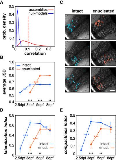
The Tectal Spontaneous Activity Structure Is Organized in Functional Neuronal Assemblies

(A) Probability (prob.) density of the distributions of the average correlations between neurons within each assembly and the corresponding null model, in intact larvae 5 dpf. The dotted lines represent the average correlation, in red for the data (0.108 ± 0.010) and blue for the null models (0.016 ± 0.002).

(B) Average JSD for the spontaneous neuronal assemblies across the different developmental stages, in intact and enucleated conditions.

(C) Topographies of representative neuronal assemblies emerging from the spontaneous activity of a 5 dpf intact and enucleated larva. Scale bar, 100 μm.

(D and E) Average index of lateralization, depicting the position of neurons within an assembly across both tecta (D), and index of compactness, representing the dispersion of neurons within a given assembly (E), for the neuronal assemblies during development, in intact and enucleated (enucl.) larvae.

Blue indicates intact larvae, and red indicates enucleated larvae in (B), (D), and (E).

^∗: p < 0.05; ^∗∗: p < 0.01; ^∗∗∗: p < 0.001. Error bars indicate SEM.

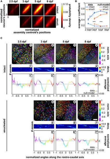
The Spontaneous Neuronal Assemblies Progressively Organize along the Tectal Caudo-rostral Axis, during Development

(A) Density plots of the caudo-rostral normalized positions of each neuron against the normalized position of each neuronal assembly centroid along the caudo-rostral axis of the tectum, in intact and enucleated (enucl.) larvae, at each developmental stage; 0 is the most rostral position and 1 is the most caudal one (in the enucleated 8-dpf larva density plot; the respective null models are in Figure S4C).

(B) Average r coefficients of the regression fit between the position of the assembly’s centroids and that of the assembly’s neurons, along the caudo-rostral axis, in intact (blue) and enucleated (enucl.; red) larvae. The respective null models are depicted by the dashed curves in the right panel. ^∗∗∗p < 0.001.

(C) Topographic organization of the spontaneous neuronal assemblies. (1–4) Examples of assemblies’ topographies projected along the caudo-rostral axis of an intact larva at different developmental stages. Color bar: position along the caudo-rostral axis (the neurons are color coded according to the centroid azimuthal position of the assembly to which they belong). (5–7) Same as for (1)–(4), but for the enucleated larvae. Scale bar represents 100 μm. (1'–7') Distribution of the density of number of neurons belonging to each assembly, along the normalized (norm.) caudo-rostral axis, for the experiment illustrated in (1)–(7), respectively; y axis: neuronal assembly number (# assem.); x axis: normalized caudo-rostral tectal axis (see Figure S4D for the distributions of all experiments and their respective null models). Color bar: neuronal density along the normalized caudo-rostral axis (dens.). (1''–7'') Average normalized mean distributions of the assemblies’ neuronal densities in (1')–(7'), for all experiments during the different developmental stages, in intact and enucleated conditions, color coded accordingly to their normalized azimuthal positions (color bar). The normalized mean distributions of the respective null models are depicted in gray.

Error bars indicate SEM. See also Figure S4.

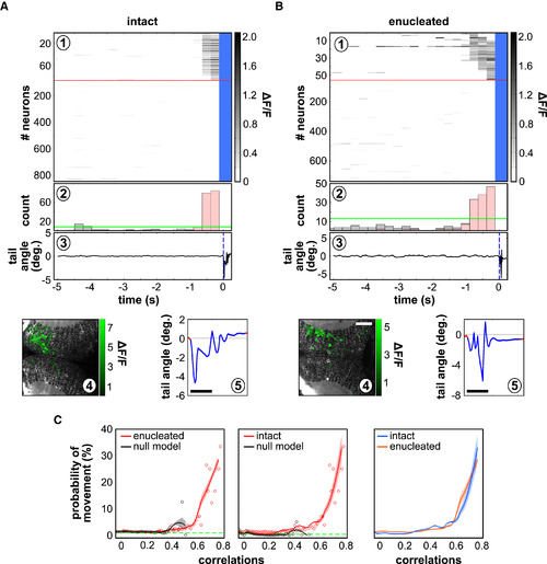
Spontaneous Neuronal Assemblies Are Predictive of Tail Motor Behaviors, even in Chronic Absence of Retinal Inputs

(A and B) Examples of spontaneous activation of a topographically compact tectal assembly before the onset of a tail movement in an intact larva (A) and an enucleated larva (B). (A1 and B1) Raster plot of all imaged tectal neurons; the red line separates the neurons belonging to the active neuronal pattern before the tail flip (above), from the rest of the neurons in the circuit (below; notice that the scale is different above and below the line; blue indicates frames during tail-flip movements). (A2 and B2) Histogram of the number of active neurons in the circuit; the fraction of neurons in the active neuronal pattern is represented in pink; the green line represents the threshold for significant neuronal population events. (A3 and B3) Tail angle. The blue dashed line indicates the onset of tail movement. Deg, degree. (A4 and B4) Topography of the spontaneously active neuronal pattern; compactness index: 0.54 (A4) and 0.33 (B4). (A5 and B5) A magnification of the angle of the tail during the movement. Scale bars, 100 ms.

(C) Probability of a tail movement as a function of the correlation between all assembly patterns and the spontaneous tectal network activity for the imaging frame preceding the movement onset in intact larvae (left; n = 6) and enucleated larvae (middle; n = 6). Red dots indicate raw data; black dots indicate null models; red curves indicate regression fits, with CI_95%; black curves indicate null-model assemblies; and dashed green lines indicate global average probability of movements. Right: comparison between intact larvae (blue) and enucleated larvae (red).

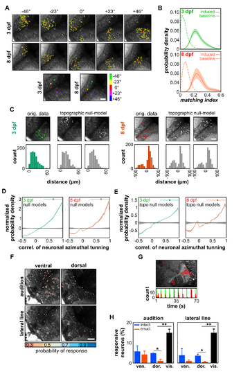
Spontaneous neuronal assemblies regroup functionally related neurons, related to Figure 2.

(A) Examples of neuronal assemblies induced by light-spots of 20° angular size, across the visual field (from -46° to +46°) at 3 and 8 dpf; the center of mass of each visually induced assembly is indicated by a red dot; these dots are color-coded in the bottom panels according to the position of the visual stimulus that induced the response. Note the match between the order of the colors along the caudo-rostral axis and the colors representing the different positions of stimulation, indicating that the tectal retinotopic map is organized along the tectal caudo-rostral axis.

(B) Probability density distributions of the MIs of the significant visually induced neuronal groups (3 dpf: green; 8 dpf: red), during the periods of spontaneous activity. The dashed curves represent the distribution of the non-significant MI values (baselines). Note that distributions and magnitudes of induced assemblies were comparable at 3 and 8 dpf: the probability density peaks of the significant matching index were 0.226 ± 0.013 at 3 dpf and 0.254 ± 0.013 at 8 dpf, while the ones of their respective baseline were 0.047 ± 0.006 (p < 10^-5 by comparing MIs and baselines) and 0.067 ± 0.004 (p < 10^-4).

(C) Examples of 3 dpf (left panels) and 8 dpf (right panels) spontaneous assemblies and corresponding two topographic null assemblies (out of 50). Notice that the distributions of the distance between pair of neurons in the assembly and their respective null model assemblies are similar (bottom panels); positive and negative distance correspond to intra- and interhemisphere neuronal pairs, respectively.

(D) Distribution of the normalized probability density of the pooled pair-wise correlation coefficients of the spatial tuning curves (azimuth tuning curves) of neurons belonging to spontaneous assemblies at 3 (green) and 8 dpf (red) and their respective null models (black). For the normalization, the distributions were divided by the null-model distributions. Note the large bias of the spontaneous assemblies toward grouping neurons with highly similar tuning curves, both at 3 and 8 dpf. The confidence intervals were calculated with a Jack-Knife procedure, across experiments. The significant bias range and median are indicated by the top line and the dot, respectively. The bias ranges became significant above 0.32 ± 0.01 and 0.26 ± 0.08, with medians of 0.633 ± 0.004 and 0.642 ± 0.003, for 3 and 8 dpf larvae respectively (the medians between stages were not statistically different: p = 0.116).

(E). Same as D, but the normalization was performed using the distribution of the topographic null-models. Remarkably, the original assemblies still had a significant bias toward neurons with similar tunings, despite the preservation of the distribution of pair-wise distances in these topographic null-models.

(F) Examples of topographic localization of the neurons responding to at least 25% of the auditory (top panels) or lateral line stimuli (bottom panels) in a ventral (left panels) and a dorsal (right panels) layer of the optic tectum. The scale bar indicates the probability of response (resp.) of the neurons to at least 25% of the stimuli.

(G) To test whether the weak tectal response to lateral line stimuli is a direct consequence of lateral line stimulation failure, we monitored the response in the torus semicircularis (TS, its neuropil is outlined by a pale dashed blue line). Regions of interest (ROIs, delineated out of a homogeneous 10 x 10 pixels grid) in red show the TS regions responding to at least 25 % of the stimuli. The histogram of the significant Ca2+ events of the ROIs show a reliable and strong response to lateral line stimuli in the TS. (H) Proportion of neurons responding to at least 25 % of the auditory (left panel) and lateral line (right panel) stimuli, in intact (n = 3, blue) and enucleated larvae (n = 3, red). The proportion of responsive neurons to visual stimulation (vis., moving bar across the visual field) in the dorsal layer of the optic tectum (n = 13, black). Note the significant large differences of the visual responses with respect to the auditory and lateral line ones (p < 0.005). In the ventral layers (vent.) of the optic tectum, we observed no significant differences between intact and enucleated larvae for auditory and lateral line responses (p > 0.97). In the dorsal layers (dor.), the proportion of cells responding to the stimulation tends however to be smaller in the enucleated than in the intact larvae (p < 0.04). Error bars: SEM.

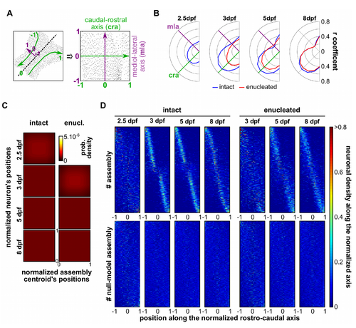
The neuronal assemblies are distributed along the caudo-rostral axis, related to Figure 3.

(A) Example of normalization of the neuronal coordinates in a common spatial reference map, where each dot represents a neuron in its original position (left) and after the normalization (right); the morphological medio-lateral (mla) and caudo-rostral axis (cra) are represented in green and purple, respectively.

(B) Correlation coefficients between the neurons belonging to each assembly and their respective centroids along different axes of the common spatial reference map, rotated every 15° for a total of 180°, for each tectum and for all developmental stages, in intact (blue) and enucleated (red) larvae. Note that the highest correlations were obtained along the tectal caudo-rostral axis in all considered conditions.

(C) Null-model density plots of the caudo-rostal normalized positions of each neuron against the normalized position of each neuronal assembly centroid, along the caudo-rostral axis of the tectum, in intact and enucleated larvae, at each developmental stage; 0 is the most rostral position and 1, the most caudal one (indicated in the enucleated 8 dpf larva density plot).

(D) Distribution of the density of the neurons per assembly along the normalized caudo-rostral axis (the axis was normalized between -1 to 1, from lateral left to lateral right) at all developmental stages, in intact (n = 622, 800, 1101 and 864 assemblies for 2.5, 3, 5 and 8 dpf stage respectively) and enucleated larvae (n = 511, 768 and 688 assemblies for 3, 5 and 8 dpf stage, respectively) and their respective null models (built from 50 repetitions of each neuronal assembly). Each neuronal assemblies are represented on the y-axis.