
- Title
-
A behavioral and modeling study of control algorithms underlying the translational optomotor response in larval zebrafish with implications for neural circuit function
- Authors
- Holman, J.G., Lai, W.W.K., Pichler, P., Saska, D., Lagnado, L., Buckley, C.L.
- Source
- Full text @ PLoS Comput. Biol.
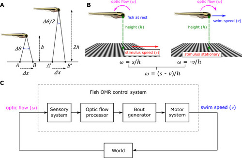
Optic flow and feedback control of the OMR.
(A) Optic flow is inversely proportional to height. The fish on the left is at rest a distance ℎ above a moving stimulus. A point on the stimulus moves forward a small distance Δx from A to B over time Δt, causing the angle of the ray passing from that point through the optical center of the eye to change by Δθ with corresponding optic flow of Δθ/Δt radians/s. The fish on the right at twice a height experiences half the change in angle, Δθ/2, for the same small stimulus movement in the same time, and thus half the optic flow. If the stimulus speed is s, Δθ = Δθ/h = sΔt/h, so the optical flow ω = Δθ/Δt = s/h. (B) Optic flow is a combination of baseline flow and swim-induced flow. As in (A), a fish at rest at height h with the stimulus below moving at speed s experiences a positive (anticlockwise) baseline optic flow of s/h rad/s when expressed as an angular velocity (left). Conversely, swimming at speed ν over a stationary grid induces a negative optic flow of -ν/h rad/s (right). When both fish and the grid are moving the opposing optic flows sum to a total of (s - ν)/h rad/s. (C). The overall system is a closed-loop feedback system with gain inversely proportional to height. Any change in the swim speed output causes a change in the optic flow input, which in turn feeds back to affect future swimming. Following [9], the system’s feedback gain can be defined as the change in optic flow caused by a small change in the swim speed taken as an index of motor effort, divided by that swim speed change, i.e., the derivative of the input with respect to the output dω/dν. The optic flow ω = (s - ν)/h, with s and h constant for any given trial, so the feedback gain dω/dν = -1/h. Like the optic flow itself, the feedback gain is inversely proportional to the height of the fish above the ground–in fact it is just the negative reciprocal of the height. |

Free swimming setup and the OMR regulation experiment.
(A) Schematic illustration of the experimental apparatus. (B) OMR regulation procedure. Each fish is tested at one of three different heights and the same set of stimulus speeds. For a given stimulus speed, baseline optic flow–the optic flow experienced when the fish is at rest–and feedback gain both decrease as the height increases. (C) Sample trace showing position of the fish from the start of the channel. The light blue points show possible positions for the center of mass at each time step; the black line shows the positions selected as most probable by the tracking algorithm from those candidates. Dotted rectangle shows region shown in (D). (D) Magnified portion of trace containing a single bout. (E) Mean swim speed and OMR ratio for the OMR regulation procedure. OMR ratio is defined as the ratio of the mean swim speed observed during OMR trajectories to the speed of the grid stimulus. Error bars here and elsewhere: standard error. (F) Bout patterns for the OMR regulation procedure. |
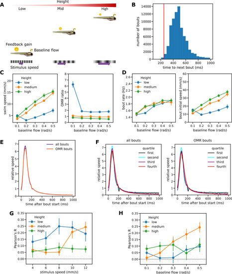
Experimental results for the baseline flow experiment and bout analysis.
(A) Baseline optical flow procedure. Each fish is tested at one of three different heights with the stimulus speed increased in proportion to height. Feedback gain decreases as the height increases but the baseline optical flow remains constant. (B) Histogram of intervals from the start of one bout to the start of the next for OMR-consistent bouts pooled from both procedures. The interval exceeded 250ms for 99.5% of bouts C) Mean swim speed and OMR ratio for the baseline flow procedure. (D) Bout patterns for the baseline flow procedure. Bout speed increased with height, but bout rate did not. (E) Overall relative bout speed profile from both experiments for all observed bouts and for OMR-consistent bouts only. The profile was not sensitive to the behavioral context. (F) Separate relative speed profiles for bouts split into quartiles by initial bout speed (swim speed averaged over the first 100ms of a bout). The relative speed profiles were essentially independent of the absolute bout speeds and again similar for all bouts (left) and OMR-consistent bouts (right). (G-H) Bout speed and time to next bout were positively correlated for OMR-consistent bouts in both the OMR regulation (G) and baseline flow procedures (H). |

Modeling I: Single process model.
Operation of the single process model. For further details see main text and the more formal model description section of the Methods. (A) Fish swimming in the same direction as a moving grid below. The resulting translational optic flow, expressed as an angular velocity, is the ratio of the difference between grid speed and swim speed and the height of the fish above the grid, as explained in Fig 1B. (B) Sample traces generated by the single factor model. The top two traces show the observable variables swim speed and optic flow; the bottom traces show three key model variables. The vertical lines show events occurring during the first bout (red, a-c), second bout (green, d-f) and third bout (magenta, g). (C) Block diagram for the single factor model. The sensed flow is a delayed version of the actual optic flow. The flow processor smooths the sensed flow by applying leaky integration and rectifies it to produce the control signal input to the bout generator. Within the bout generator, the amplified control signal drives an impulse generator that implements a Poisson process for the event of bout initiation. The same control signal also modulates the amplitude of the initiating impulses from the impulse generator to produce scaled impulses input to the profile generator. The profile generator in turn generates a swim bout that starts when the scaled impulse is received and whose speed follows the fixed relative swim speed profile observed scaled up by the amplitude of the scaled impulse. The model has three parameters to fit to data: the time constant for leaky integration (τf) and the gains applied to the control signal to determine the Poisson rate for bout initiation events (kr) and the amplitude of scaled impulses (ki). (D-E) Comparison of swim speeds and degrees of regulation as observed in the experiments and predicted by the single factor model when fitted to mean observed swim speeds for the OMR regulation procedure (D) and the baseline flow procedure (E). |
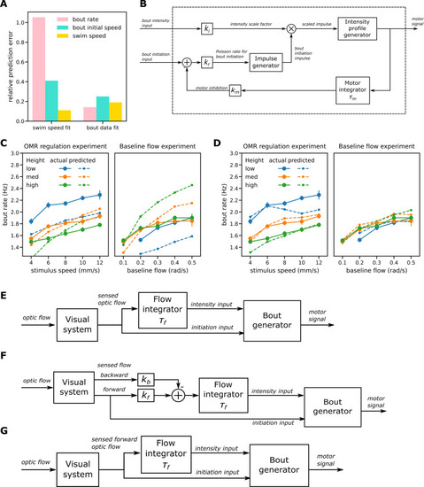
Modeling II: enhanced bout generation and two-factor model.
(A) Mean prediction errors for the single factor model fitted to mean swim speed (left group of bars) and to bout measures (mean bout rate and intensity) (right group). Fitting to swim speed failed to predict the bout measures; fitting to bout data reduced prediction errors for bout measures but produced less accurate swim speed predictions. (B) Enhanced bout generator has separate inputs for bout intensity and bout initiation and the latter is subject to motor inhibition. (C) Bout rates for the single factor model fitted to bout measures. The model failed to predict that bout rates are sensitive to height in the OMR regulation procedure (left) but not the baseline flow one (right). (D) Bout rates predicted by the enhanced bout generator when fitted to bout data and constrained to reproduce the observed bout intensities. It was now possible to reproduce the bout rate patterns observed in the two experiments. (E-G) Dual factor model variants. Each variant has an enhanced bout generator with separate bout intensity and initiation inputs. Optic flow is integrated only for the intensity input. (E) Variant A: the overall optic flow is integrated. (F) Variant B: input to the flow integrator is a linear combination of the forward and backward components of optic flow. (G) Variant C: only the forward component of the optic flow participates in control of the translational OMR. |

Modeling III: performance of dual factor model.
(A) Relative prediction errors for the basic single factor model and the three variants of the dual factor model. All variants of the dual factor model predicted both bout measures and swim speeds better than the single factor model. Variant C that processes only forward flow gave lower prediction errors than variant A and similar ones to the more general variant B, suggesting its adoption as the preferred model. (B-C) Comparison of observed bout rates, bout speeds and mean swim speeds with those predicted by variant C of the dual process model. In general, a good fit is achieved to the observed values for both OMR regulation (B) and the baseline flow procedures (C). (D) Sample signal traces generated by variant C of the two-factor model when height is intermediate (32mm) and stimulus speed 8 mm/s. Red dotted lines indicate times of bout initiation. |