Fig. 1. Clock genes expression in the zebrafish habenula based on single cell RNA sequencing A) Dot plot showing mean log-normalized expression per cluster and percentage of cells per cluster expressing each gene in the SmartSeq-2 dataset from Pandey et al. B) t-SNE representation of clustering results in the SmartSeq-2 dataset. Each point is a cell. C) same as A) but in the 10X dataset. D) same as C but in the 10X dataset. The cluster assignment for the 10X dataset corresponds to those assigned by Pandey et al., (2018).

Fig. 2. Dynamics of clock gene expression in the zebrafish habenula. (A–C). Single optical sections of the brain of 6 day old larvae fixed at six different time points, labelled for arltn1b (A) and per3 (A) using hybridization chain reaction. (C) Merge of (A) and (B). Arrowheads indicate the habenula. (D) Ratio of arntl1b/per3 in the habenula of fish in a normal LD cycle. (E-G) Expression of per3 and arntl1b in the habenula of fish grown under DD conditions. (H–N) cry1a expression in the habenula of fish grown under DD conditions. Images in E and F are maximum projections of the entire habenula. Images in panels H–M are maximum projections spanning 5 μm. The arrowheads indicate autofluorescent blood cells. A, B, C, E, F, H-M are dorsal views with anterior to the top. The dots in panels D, G and N indicate values for individual fish. The horizontal bars indicate illumination conditions. lHb: left habenula; rHb: right habenula; Pi: pineal; Pa: pallium; OT: optic tectum. Scale bar = 25 μm.

Fig. 3. Circadian variation in cytoplasmic calcium in habenula neurons. (A-E) Long duration multiplane recording of the habenula of Et(GAL4s1011t),Tg(UAS:GCaMP6s) larvae in constant darkness. (A–D) Examples of imaging data from one fish at two different time points, ZT5 (A, B) and ZT14 (C, D), and two different focal planes, dorsal (A, C) and ventral (B, D). Scale bar = 25 μm, dorsal view with anterior to the top. The wedge shows the look up table (LUT) used to represent pixel intensities, with values ranging from 3 (blue) to 3939 (red). (E) Average level of cytoplasmic calcium in the habenula, as shown by intensity of GCaMP6s. Each coloured trace represents a different fish. The thicker black line is the mean. There is a reduction in intracellular calcium levels during the subjective night and an increase in the subjective day. The dotted brown line is a sine wave that the data was regressed to, with an R² of 0.869. (F–G) Difference in relative activity levels of habenula neurons between day (ZT3) and night (ZT15) as measured by both cytoplasmic and nuclear GCaMP6s. (F) Distribution of the mean of vectors containing z-scores of neurons with high variance in their activity. The distributions are different, as determined by Kolmogorov-Smirnov test, with p < 0.0001. (G) K-means cluster distribution for the same vectors. P < 0.0001 by Chi-squared test. (For interpretation of the references to colour in this figure legend, the reader is referred to the Web version of this article.)

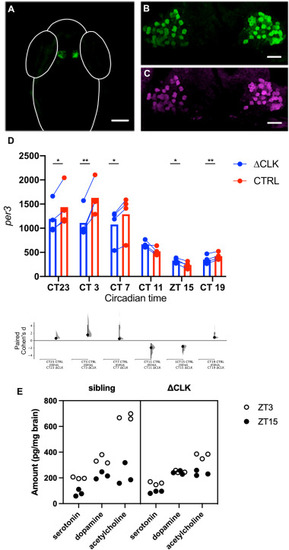
Fig. 4. The effects of expressing truncated clocka in the habenula. (A) Specific expression of EGFP in the habenula of a Tg(gng8:GAL4, UAS:EGFP-Δclocka) fish. (B) At higher magnification, EGFP is visible in the cytoplasm of habenula neurons. (C) Detection of Myc, which is fused to the C-terminus of ΔCLK, in the habenula of transgenic fish. (D) Level of per3 in the habenula of fish with mosaic expression of EGFP-ΔCLK, as determined by qHCR imaging. The lower graph shows Cohen's d, indicating the degree of difference between ΔCLK-expressing and non-expressing cells at each time point. Values are given in the main text. (E) Effects of ΔCLK expression in the habenula on global neuromodulator levels. Plot showing the amount of secreted serotonin, dopamine and acetylcholine in the whole brain of and Tg(gng8:GAL4, UAS:EGFP-Δclocka) and sibling fish (N = 3) at ZT3 and ZT15. Fish with ΔCLK expression in the habenula have a reduced day-night change in levels. Scale bar = 100 μm in panel A, 20 μm in panels B and C; * indicates p < 0.05; ** indicates p < 0.005 by paired t-test. Exact p values are provided in the text.

Fig. 5. The effects of the alarm substance Schreckstoff on Tg(gng8:GAL4, UAS:EGFP-Δclocka) fish. (A–D) Acute effects in adult fish (N = 12). (A) Schematic diagram of the experiment. (B) Speed distribution in fish before and after exposure to the alarm substance, where the substance remained in the tank after delivery. (C–D) Time spent darting (C), restricted to the tank base (D) in the presence of the alarm substance. As indicated by the paired mean difference plots (lower plot), fish with and without expression of truncated clocka behave similarly. (E–G) Post-exposure behaviour in adult fish (N = 8). (E) Schematic diagram of the experiment. (F) Speed distribution in a novel tank containing clean water, after exposure to alarm substance or clean water. (G) Distance traversed in a novel tank containing clean water, at different times after exposure to the alarm substance. (H–J) Post-exposure behaviour in 2 week-old zebrafish. (H) Schematic diagram of the experiment. (I) Percentage of time in the dark area of a tank, after 10 min of exposure to embryo water. (J) Percentage of time spent in the dark side after exposure to the alarm substance. Tg(gng8:GAL4, UAS:EGFP-Δclocka) fish spend more time in the dark side, with a Cohen's D of 1.2.

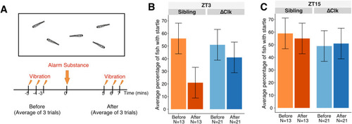
Fig. 6. Day-night variation in the response of zebrafish to Schreckstoff. (A) Schematic diagram of the experiment. To assess freezing in larval fish following exposure to the alarm substance, fish were exposed to vibrations in the day (ZT3) (B) or at night (ZT15) (C). Control fish, which are non-expressing siblings of Tg(gng8:GAL4, UAS:Δclocka) fish, show a reduction in startle after exposure during the day, but not at night. This response to alarm substance was not seen in Tg(gng8:GAL4, UAS:Δclocka) fish in the day or night. Error bars in panels B and C indicate standard deviation.

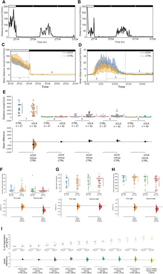
Fig. 7. Sleep is unaltered in Tg(gng8:GAL4, UAS:EGFP-Δclocka) larvae

(A, B) Distances moved (cm/10 min) by an individual fish from (A) Control group and (B) ΔCLK group, plotted against time (hr) over the time-course of the whole recording. CT = circadian time. (C, D) Mean distances moved (cm/10 min) of ΔCLK (blue) and control (orange) groups, plotted against time (hr) (C) during the first 14 h of recording, including 4 h of light-phase and 10 h in the dark during the night (i.e. Zeitgeber Time ZT 10–14 and ZT 14–24) and (D) during the subsequent 24 h of recording under DD (i.e. Circadian Time CT 0–24). 95% CIs are indicated by the shaded areas; horizontal brackets indicate 5 timeframes analysed in panel E. Black and white bars represent periods of dark and light, respectively. (E) The Cumming estimation plot shows the mean differences in 5 timeframes of the recording: ZT10-14 (1; light-phase), ZT14-24 (2; first night), CT0-7 (3: early subjective day), CT7-14 (4: late subjective day) and CT14-24 (5: subjective night). The upper axis shows the raw data, with each dot representing the overall distance moved (cm) by a single larva; gapped vertical lines to the right of each group indicate mean ± SD. Each mean difference is plotted on the lower axes as a bootstrap sampling distribution. Mean differences are depicted as black dots and 95% CIs are indicated by the end of vertical error bars. (F–H) Analysis of sleep during the subjective night. ΔCLK and control fish have similar average sleep bout (F), sleep bout frequency (G) and total sleep (H). (I) Analysis of sensory responsiveness of the Tg(gng8:GAL4, UAS:EGFP-Δclocka) larvae (7 dpf) during the delivery of auditory stimuli of 9 different intensities. The Cumming estimation plot shows the mean differences for 9 comparisons, corresponding to 9 stimulus intensities (0–100%). The raw data is plotted on the upper axis, each dot representing the percentage of responders per single experimental run. . (For interpretation of the references to colour in this figure legend, the reader is referred to the Web version of this article.)