
|
Fig. 4
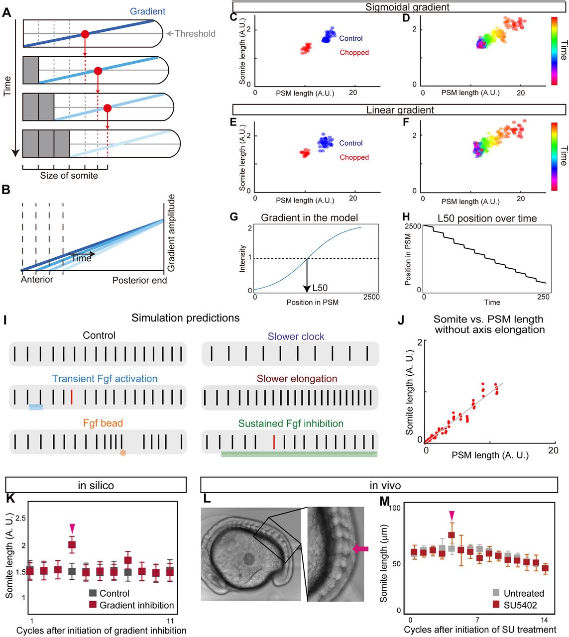
Clock and scaled gradient model. (A) Schematic of the clock and scaled gradient model. The position of a future somite boundary is set by a scaled gradient once per clock cycle (each row) and the boundary appears after a delay. (B) Superimposition of the gradients from each time point shown in A. (C,D) Simulation results using a sigmoidal gradient. (E,F) Simulation results using a linear gradient. (C,E) Simulation results of control and chopped embryos. (D,F) Simulation results of a single embryo over time. (G,H) Stepwise regression of the gradient in clock and scaled gradient model. (G) L50 in the model was determined similarly to Fig. 3P. (H) Clock and scaled gradient model predicts stepwise regression of L50 position. (I) Simulation results for perturbation experiments for local or global inhibition/activation of Fgf, slower clock and slower axis elongation. Black vertical lines represent simulated somite boundary positions. (J) Somite size versus PSM length shows perfect scaling in silico when axial elongation speed is zero, mimicking the results from the in vitro mPSM system (Lauschke et al., 2013). (K) Simulation results of long-term suppression of a gradient in the clock and scaled gradient model. Error bars denote s.d. (L,M) Treatment with a low concentration of SU5402 (16 μM) results in one or two larger somite(s) (arrow) (n=7 for both SU5402 and untreated groups). Error bars denote s.d.