
- Title
-
A simple and effective F0 knockout method for rapid screening of behaviour and other complex phenotypes
- Authors
- Kroll, F., Powell, G.T., Ghosh, M., Gestri, G., Antinucci, P., Hearn, T.J., Tunbak, H., Lim, S., Dennis, H.W., Fernandez, J.M., Whitmore, D., Dreosti, E., Wilson, S.W., Hoffman, E.J., Rihel, J.
- Source
- Full text @ Elife
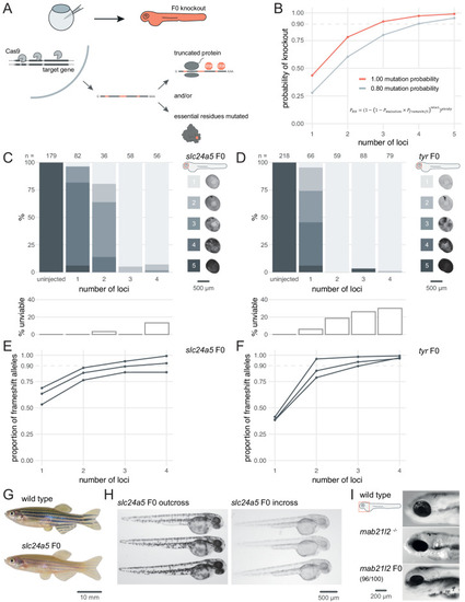
Three synthetic gRNAs per gene achieve over 90% biallelic knockouts in F0. (A) Schematic of the F0 knockout strategy. Introduction of indels at multiple loci within the target gene leads to frameshift and premature stop codons and/or mutation of essential residues. (B) Simplified theoretical model of biallelic knockout probability as a function of number of targeted loci, assuming frameshift is the sole knockout mechanism. PKO, probability of biallelic knockout; Pmutation, mutation probability (here, 1.00 or 0.80); Pframeshift, probability of frameshift after mutation (0.66); nloci, number of targeted loci. (C–D) (top) Phenotypic penetrance as additional loci in the same gene are targeted. Pictures of the eye at 2 dpf are examples of the scoring method. (bottom) Unviability as percentage of 1-dpf embryos. (E–F) Proportion of alleles harbouring a frameshift mutation if 1, 2, 3, or 4 loci in the same gene were targeted, based on deep sequencing of each targeted locus. Each line corresponds to an individual animal. (G) 2.5-month wild-type and slc24a5 F0 knockout adult fish (n = 41). (H) 2-dpf progeny from slc24a5 F0 adults outcrossed to wild types (n = 283) or incrossed (n = 313). (I) Example of 3-dpf wild type, mab21l2u517 mutant, and mab21l2 F0 embryos (n = 96/100 injected). See also Figure 1—figure supplement 1. PHENOTYPE:
|
( |
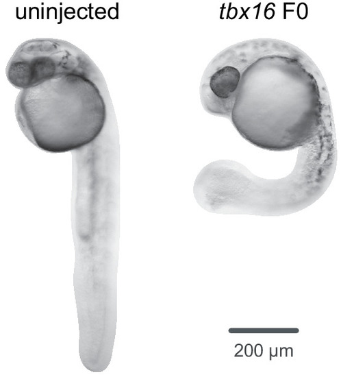
Example of 1-dpf uninjected (n = 110) and |
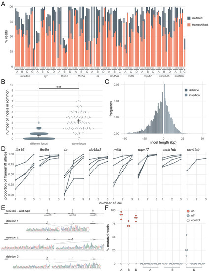
(A) Percentage of reads mutated (height of each bar, grey) and percentage of reads with a frameshift mutation (orange) at each gene, locus (capital letters refer to IDT’s database), larva (within each gene, the same number refers to the same individual animal; 0 is uninjected control). (B) Number of indels in common when intersecting the top 10 most frequent indels of two samples from different loci or from the same locus but different animals. Black crosses mark the means. *** p < 0.001; Welch’s t-test. (C) Frequency of each indel length (bp). Negative lengths: deletions, positive lengths: insertions. (D) Proportion of alleles harbouring a frameshift mutation if 1, 2, or three3 loci in the same gene were targeted, based on deep sequencing of each targeted locus. Each line corresponds to an individual animal. (E) Sanger sequencing of amplicons spanning multiple targeted loci of slc24a5. Arrowheads indicate each protospacer adjacent motif (PAM), capital letters refer to the crRNA/locus name. (F) Deep sequencing of the top 3 predicted off-targets of each slc24a5 gRNA (A, B, D). Each data point corresponds to one locus in one animal. Percentage of mutated reads at on-targets is the same data as in A (slc24a5 loci A, B, D). See also Figure 2—figure supplement 1. |
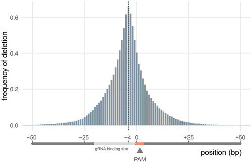
Nucleotide positions are given in relation to the protospacer adjacent motif (PAM), whose position is set at 0 (0 = PAM nucleotide adjacent to the gRNA binding site). The nucleotide 4 bp before the PAM (−4) was the most frequently deleted (67% of all deletions removed it). n = 4016 unique deletions. |
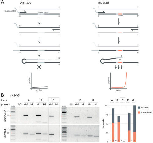
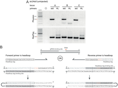
(A) Principle of headloop PCR. A headloop tag complementary to the target locus is added to one PCR primer (here, to the forward primer). During PCR, the first elongation incorporates the primer and its overhang; the second elongation synthesises the headloop tag. (left) If the template is wild-type, the complementary tag base-pairs with the target locus and directs elongation (hatched sequence). The amplicon forms a hairpin secondary structure, which prevents its subsequent use as template. (right) If the targeted locus is mutated, the tag is no longer complementary to the locus. The amplicon remains accessible as a template, leading to exponential PCR amplification. (B) (left) Target loci (A, B, C, D, G) of slc24a5 amplified with the PCR primers used for sequencing (std, standard) or when one is replaced by a headloop primer (HL). Orange arrowheads mark the 300 bp ladder band. (right) Deep sequencing results of the same samples as comparison (reproduced from Figure 2A, except locus C); u, uninjected control, i, injected embryo. Framed are results for gRNA C, which repeatedly failed to generate many mutations. See also Figure 3—figure supplement 1, 2, 3. |
( |
( |
( |
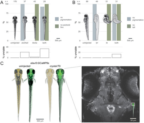
(A) Penetrance of single (slc24a5, tbx5a) and combined (both) biallelic knockout phenotype(s) in F0. Pictures of example larvae were taken at 3 dpf. No pigmentation refers to embryos clear of eye pigmentation at 2 dpf, as in Figure 1C. Pectoral fins were inspected at 3 dpf. (bottom) Unviability as percentage of 1-dpf embryos. (B) Penetrance of single (tyr, ta) and combined (both) biallelic knockout phenotype(s) in F0. Pictures of example larvae were taken at 2 dpf. (bottom) Unviability as percentage of 1-dpf embryos. (C) (left) Pictures of example elavl3:GCaMP6s larvae at 4 dpf. Left was uninjected; right was injected and displays the crystal phenotype. Pictures without fluorescence were taken with illumination from above to show the iridophores, or lack thereof. (right) Two-photon GCaMP imaging (z-projection) of the elavl3:GCaMP6s, crystal F0 larva shown on the left. (inset) Area of image (white box). See also Figure 4—video 1, Figure 4—video 2. PHENOTYPE:
|
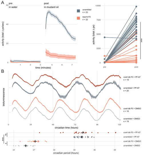
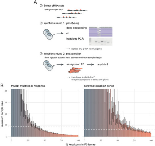
(A) Escape response to mustard oil in trpa1b F0 knockouts. (left) Activity (total Δ pixel/second) of scrambled controls and trpa1b F0 knockout larvae at 4 dpf. Pre: 3-min window before transfer to 1 µM mustard oil. Post: 3-min window immediately after. Traces are mean ± standard error of the mean (SEM). (right) Total activity (sum of Δ pixel/frame over the 3-min window) of individual larvae before and after transfer to 1 µM mustard oil. *** p < 0.001 (Δ total activity scrambled vs trpa1b F0); Welch’s t-test. (B) Circadian rhythm quantification in csnk1db F0 knockout larvae. (top) Timeseries (detrended and normalised) of bioluminescence from per3:luciferase larvae over five subjective day/night cycles (constant dark). Circadian time is the number of hours after the last Zeitgeber (circadian time 0 9 am, morning of 4 dpf). DMSO: 0.001% dimethyl sulfoxide; PF-67: 1 µM PF-670462. Traces are mean ± SEM. (bottom) Circadian period of each larva calculated from its timeseries. Black crosses mark the population means. ns, p = 0.825; * p = 0.024; *** p < 0.001; pairwise Welch’s t-tests with Holm’s p-value adjustment. See also Figure 4—video 1. PHENOTYPE:
|
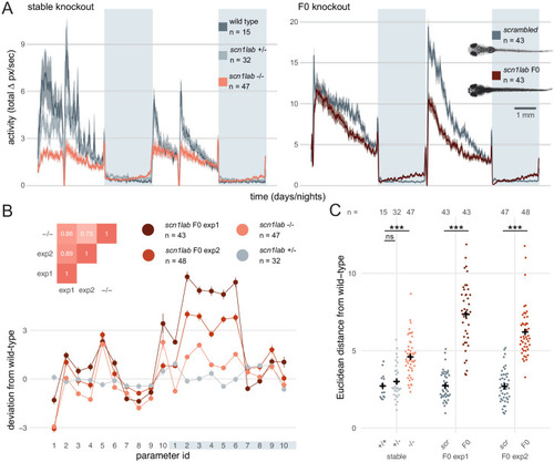
(A) Activity (total Δ pixel/second) of larvae across 2 days (14 hr each, white background) and two nights (10 hr each, grey background). Traces are mean ± SEM. (left) Stable scn1labΔ44 mutant line, from 5 to 7 dpf. The drops in activity in the middle of each day is an artefact caused by topping-up the water. (right) scn1lab F0 knockout, from 6 to 8 dpf. This replicate is called scn1lab F0 experiment 1 in B and C. (inset) Pictures of example scrambled-injected control and scn1lab F0 larvae at 6 dpf. (B) Behavioural fingerprints, represented as deviation from the paired wild-type mean (Z-score, mean ± SEM). 10 parameters describe bout structure during the day and night (grey underlay). Parameters 1–6 describe the swimming (active) bouts, 7–9 the activity during each day/night, and 10 is pause (inactive bout) length. (inset) Pairwise correlations (Pearson) between mean fingerprints. (C) Euclidean distance of individual larvae from the paired wild-type or scrambled-injected (scr) mean. Black crosses mark the population means. ns, p > 0.999; *** p < 0.001; pairwise Welch’s t-tests with Holm’s p-value adjustment. See also Figure 6—figure supplement 1. |
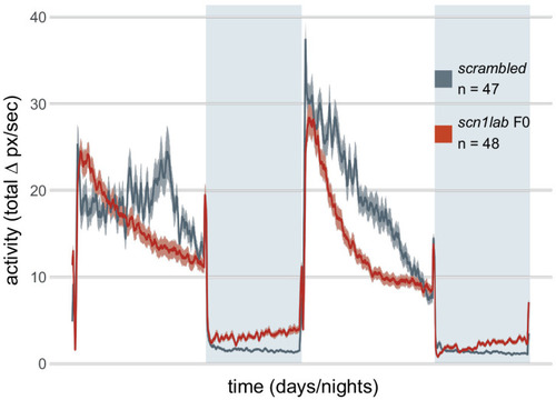
This replicate is called |
( |