(A) Spectral clustering (scikit-learn) was used to cluster the continuous eye angle over each bout for both eyes. The initiation of hunt sequences was identified using Cluster three and deconvergence of the eyes was demarked by Cluster 1. (B) Hunt sequence types in the dataset. The user’s only role is to denote the last bout of the hunt sequence, characterize the sequence as a strike hit, strike miss, or abort, and note the chosen prey ID assigned by our automated prey reconstruction algorithm. The program then outputs the descriptors in B per hunt. ‘Collisions’ imply that the fish head has collided with the wall during the hunt (detected using fish COM and edge coordinates), preventing analysis of whether the fish would have struck or aborted. Collisions with unknown target are likely hunting of a paramecium reflection. Deconvergence, known target and unknown target, is the standard abort described previously (Johnson et al., 2019; Henriques et al., 2019), with ‘unknown targets’ being too ambiguous for the user to make a call on pursued prey ID. No deconvergence, known target are hunts where fish had initiated to and pursued a particular prey item, but clearly stopped pursuit on a particular bout not assigned to Cluster 1. ‘Probably not a hunt’ was a rare case where the fish converged, swam through the tank without choosing a prey, and did not deconverge within eight bouts. ‘Strike at Nothing’ was another rare case where the fish converged and struck without a prey item present. The fish did spend some time striking at immobile objects that were almost invariably residue stuck to the top of the tank. During strike hits, fish choose a prey and consume it, with strike misses typically a deflection of the prey off the fish’s mouth at hunt termination. The main manuscript is built off of strike hits and misses (which combined into a ‘strikes at known prey’ category would be the most common outcome), while Supplementary Figure 3’s abort algorithm is built from known target, deconverge and no-deconverge hunts. Collisions are simply an outcome of having a relatively small tank for parfocal imaging compared to the fish’s real environment; hunts resulting in collisions were not analyzed except for the initial choice.

(A) Spectral clustering (scikit-learn) was used to cluster the continuous eye angle over each bout for both eyes. The initiation of hunt sequences was identified using Cluster three and deconvergence of the eyes was demarked by Cluster 1. (B) Hunt sequence types in the dataset. The user’s only role is to denote the last bout of the hunt sequence, characterize the sequence as a strike hit, strike miss, or abort, and note the chosen prey ID assigned by our automated prey reconstruction algorithm. The program then outputs the descriptors in B per hunt. ‘Collisions’ imply that the fish head has collided with the wall during the hunt (detected using fish COM and edge coordinates), preventing analysis of whether the fish would have struck or aborted. Collisions with unknown target are likely hunting of a paramecium reflection. Deconvergence, known target and unknown target, is the standard abort described previously (Johnson et al., 2019; Henriques et al., 2019), with ‘unknown targets’ being too ambiguous for the user to make a call on pursued prey ID. No deconvergence, known target are hunts where fish had initiated to and pursued a particular prey item, but clearly stopped pursuit on a particular bout not assigned to Cluster 1. ‘Probably not a hunt’ was a rare case where the fish converged, swam through the tank without choosing a prey, and did not deconverge within eight bouts. ‘Strike at Nothing’ was another rare case where the fish converged and struck without a prey item present. The fish did spend some time striking at immobile objects that were almost invariably residue stuck to the top of the tank. During strike hits, fish choose a prey and consume it, with strike misses typically a deflection of the prey off the fish’s mouth at hunt termination. The main manuscript is built off of strike hits and misses (which combined into a ‘strikes at known prey’ category would be the most common outcome), while Supplementary Figure 3’s abort algorithm is built from known target, deconverge and no-deconverge hunts. Collisions are simply an outcome of having a relatively small tank for parfocal imaging compared to the fish’s real environment; hunts resulting in collisions were not analyzed except for the initial choice.

(A) Colors are histograms of coordinates for prey chosen at hunt initiation, gray are all prey records [chosen + ignored. Note: XY records passing a threshold length and velocity that remain unpaired after prey reconstruction are assigned the Z-coordinate of the tank ceiling because live paramecia show anti-gravitaxis (Roberts 2010); we always noted that a subset of prey gather at the ceiling and never noticed coagulation of prey on the ground unless dead; results are very similar to those shown if ceiling assigned prey are not counted]. (B) Histograms showing the distribution of spherical velocities for chosen prey do not reveal a bias in magnitude or direction. (C) Count plots of distance rank for selected prey (0 = closest). (D) We virtually displaced fish coordinates at hunt initiation bouts into randomly recorded paramecium environments and asked whether the closest prey item in that environment shared azimuth and altitude features with prey that fish actually chose. Histograms of the closest prey in random prey environments and prey environments in which initiation actually occurred are plotted in red (for random condition, fish orientation and position at hunt initiation is projected into a different time during the experiment; left panel). Blue (az) and yellow (alt) histograms are chosen prey histograms from (A) for comparison. The closest prey item in a random environment does not show the same distribution as selected prey in (A), indicating that the closest prey does not necessarily have to share the altitude and azimuth features of chosen prey. This suggests that somewhat specific prey features are preferred for entry into the hunting state, although transition probabilities governing hunting mode entry are also at play (Johnson et al., 2019; Mearns et al., 2019).

Figure 1—figure supplement 2—source data 1.

(A) Regression fits between prey position and bout variables during hunt sequences ending in an abort. Gray points and lines represent the last three pursuit bouts before the quit bout occurs, colors are all bouts between initiation and the last 3. The algorithm strongly resembles Figure 2 transformations at the beginning of hunt sequences that will eventually end in aborts, but goes awry in the last three bouts before quitting. (B) Pursuit bouts during abort sequences show modulation by velocity at inflection points similar to Figure 3—figure supplement 1B. (C) Orange model is the same as Figure 4 (Orange Model 2), which issues bouts based on multiple regression to prey position variables only. Green model is same as Figure 4 (Green Model 3), which issues bouts based on multiple regression to prey position and velocity variables. However, both are fit using pursuit bouts during aborted sequences (outside of the last three bouts before quitting) instead of strike sequences (i.e. Figure 4). As with models fit on strike sequences, multiple regression using prey position and velocity outperforms position only regression due to proportional velocity modulation. Both models are fed the exact same prey trajectories as models in Figure 4. Fitting on pursuit bouts during aborted sequences thus shows similar performance levels to models fit on strike sequences.

(A) Regression fits between prey position and bout variables during hunt sequences ending in an abort. Gray points and lines represent the last three pursuit bouts before the quit bout occurs, colors are all bouts between initiation and the last 3. The algorithm strongly resembles Figure 2 transformations at the beginning of hunt sequences that will eventually end in aborts, but goes awry in the last three bouts before quitting. (B) Pursuit bouts during abort sequences show modulation by velocity at inflection points similar to Figure 3—figure supplement 1B. (C) Orange model is the same as Figure 4 (Orange Model 2), which issues bouts based on multiple regression to prey position variables only. Green model is same as Figure 4 (Green Model 3), which issues bouts based on multiple regression to prey position and velocity variables. However, both are fit using pursuit bouts during aborted sequences (outside of the last three bouts before quitting) instead of strike sequences (i.e. Figure 4). As with models fit on strike sequences, multiple regression using prey position and velocity outperforms position only regression due to proportional velocity modulation. Both models are fed the exact same prey trajectories as models in Figure 4. Fitting on pursuit bouts during aborted sequences thus shows similar performance levels to models fit on strike sequences.

(A) Distribution of 3D velocities of prey hunted by fish in our study. Mean azimuth and altitude velocities (absolute value) are shown in reference to the fish, averaged over 80 ms before pursuit bout initiation, which is the time interval of all velocity calculations implemented here. (B) Example histograms for two 5° windows of prey space, as shown in Figure 3A,B. Again, light colors indicate that prey are moving away from the fish and dark moving toward. If prey are 0–5° to the right of the fish, but swimming toward the fish in azimuth, the fish will actually turn and displace left, predicting that the prey will cross its midline. If swimming away, fish turn and displace to the right. In a window 15–20° above the fish in altitude, the fish will actually ‘wait’ for prey with downward velocity (i.e. Bout Alt ~0°), anticipating that the prey will arrive in the strike zone. Otherwise if prey are moving upwards, fish displace and rotate upwards.

(A) Distribution of 3D velocities of prey hunted by fish in our study. Mean azimuth and altitude velocities (absolute value) are shown in reference to the fish, averaged over 80 ms before pursuit bout initiation, which is the time interval of all velocity calculations implemented here. (B) Example histograms for two 5° windows of prey space, as shown in Figure 3A,B. Again, light colors indicate that prey are moving away from the fish and dark moving toward. If prey are 0–5° to the right of the fish, but swimming toward the fish in azimuth, the fish will actually turn and displace left, predicting that the prey will cross its midline. If swimming away, fish turn and displace to the right. In a window 15–20° above the fish in altitude, the fish will actually ‘wait’ for prey with downward velocity (i.e. Bout Alt ~0°), anticipating that the prey will arrive in the strike zone. Otherwise if prey are moving upwards, fish displace and rotate upwards.

(A) A virtual prey capture environment mimicking the prey capture tank was generated to test three different types of models, and six models overall, described in the schematic. Models control a virtual fish consisting of a 3D position (red dot) and a 3D unit vector pointing in the direction of the fish’s heading. Virtual fish are started at the exact position and rotation where fish initiated hunts in the dataset. Prey trajectories are launched that reconstruct the real paramecium movements that occurred during hunts. The virtual fish moves in bouts timed to real life bouts, and if the prey enters the strike zone (defined by the distributions in Figure 2B, Materials and methods), the hunt is terminated. (B) Barplots (total #) and box plots (median and quartiles) showing performance of all six models in success (# Strikes), energy use per hunt sequence, and how many bouts each model performed during the hunt (a metric of hunt speed). (C) KDE plots showing the distribution of Post-Bout Prey Az and Post-Bout Prey Alt distributions for each model during virtual hunts. Dotted lines demark the strike zone mean.

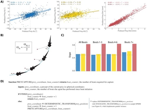
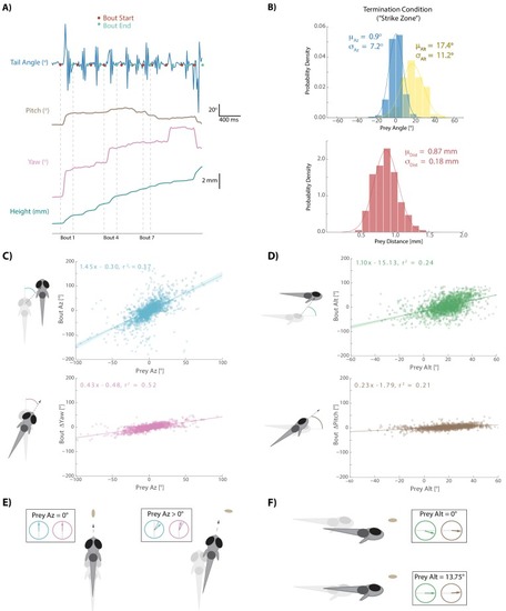
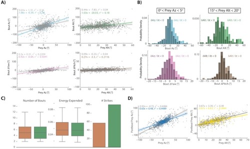
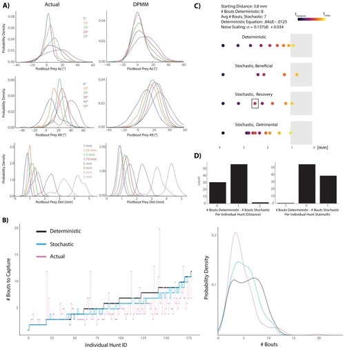
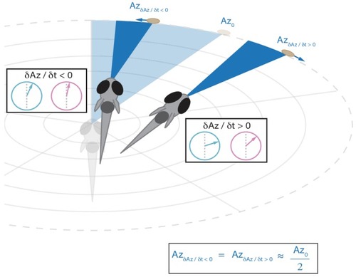
This strategy emerges from the position transforms in Figure 2 and the modulation of rotation and displacement by prey velocity in Figure 3 (Bout ΔYaw, pink wheel; Bout Az, blue wheel).

This strategy emerges from the position transforms in Figure 2 and the modulation of rotation and displacement by prey velocity in Figure 3 (Bout ΔYaw, pink wheel; Bout Az, blue wheel).

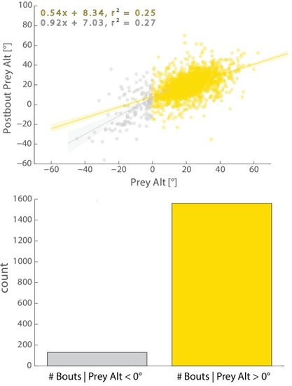
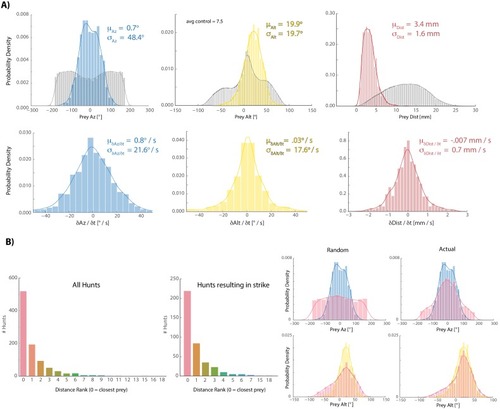
Most bouts in the dataset (>92%) occur when prey are above the fish. This change when prey cross 0° Alt is accounted for in all algorithms (see Appendix).

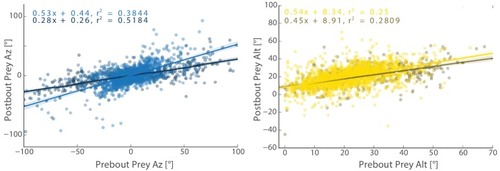
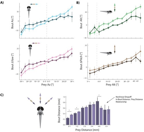
The initiation bout is a large angle turn that divides azimuth more than a pursuit bout; altitude is also significantly more reduced by the initiation bout. All regression models in simulations therefore use an independent regression fit to initiation bouts to start every simulated hunt.