
- Title
-
Linking Neurons to Network Function and Behavior by Two-Photon Holographic Optogenetics and Volumetric Imaging
- Authors
- Dal Maschio, M., Donovan, J.C., Helmbrecht, T.O., Baier, H.
- Source
- Full text @ Neuron
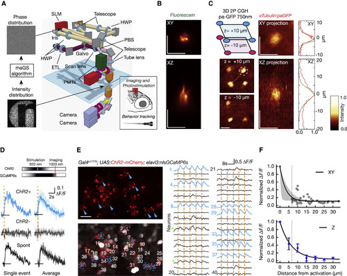
Parallel 2P Optogenetic Stimulation and Activity Readout (A) Complex illumination patterns are obtained in the sample volume using computer-generated holography (CGH). A fast Fourier transform (FFT)-based algorithm (maGS) calculates the phase modulation that generates the desired pattern at the sample plane (logo of our institute). The photostimulation path (light brown) uses a spatial light modulator (SLM) (red) to apply phase corrections. The imaging path (magenta) includes an electrically tunable lens (ETL) for remote focusing. The two paths are combined with a polarizing beam splitter (PBS) (details in Figure S1 and STAR Methods). (B) Measurement of the excitation profile obtained from a thin fluorescein layer illuminated with a circular spot 6 μm in diameter. (C) Parallel 2P activation of paGFP in vivo using a 3D excitation pattern with a distribution of circular ROIs (6 μm in diameter). The photoactivation foci are generated in the optic tectum at a depth of about 100–120 μm in a zebrafish larva with pan-neuronal paGFP expression (alpha-tubulin:paGFP). Four spots are generated at +10 μm and three spots at −10 μm. Axial and lateral average projections of a photoactivation volume obtained in vivo with a target pattern 6 μm in diameter are shown. The paGFP profiles (FWHM: 5.79 ± 0.91 μm laterally and 8.9 ± 0.9 μm axially) were photoactivated at 750 nm with a power of 0.25 mW/μm2 at the sample for 0.5 s. The right panel shows a comparison of the fluorescence profile measured for paGFP photoconversion (in red) and for a fluorescein layer (in green). (D) Somatic GCaMP6s signals induced by 200 ms photostimulation at 920 nm while imaging at 1,020 nm. Cells expressing ChR2 and GCaMP6s show stimulation-induced calcium increases (blue traces) whereas cells expressing only GCaMP6s (gray traces) do not. Activation events in targeted neurons show similar response dynamics to spontaneous events (black traces; Figures S6A and S6B). (E) Parallel neuronal stimulation in vivo. A small network of neurons is imaged during repeated simultaneous photostimulation of eight targeted neurons (in blue). Photostimulation events (200 ms) are indicated by orange vertical lines, and the traces for photostimulated neurons are in blue. Along with the targeted neurons, some cells show low-amplitude activity locked to the stimulation (green asterisk; see also Figures S6E and S6F). (F) Effective photostimulation resolution. To measure lateral resolution, targeted cells were photostimulated while nearby neurons in the same imaging plane were recorded. Each gray dot represents a non-targeted cell, with ΔF/F normalized relative to the response in the targeted cell. An exponential decay fit is shown (black line) with 95% confidence interval (bootstrap; shown in gray). The thin dashed line shows the minimum distance between cells in this region of the brain. To measure axial (Z) resolution, the imaging plane was shifted axially from the target with the ETL. An example of the protocol is shown in Figures S6G and S6H. Induced ΔF/F is normalized relative to the photostimulated target cell. In blue, an exponential fit is shown, and error bars indicate the SEM. The scale bars represent 10 μm. |
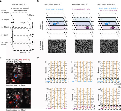
In Vivo 3D High-Resolution Photostimulation and Calcium Imaging (A) Multiplane imaging protocol. An ETL is used to switch rapidly between five imaging planes separated by 8 μm and to record GCaMP6s signals across a volume of 160 × 80 × 32 μm3 at 4 Hz. (B) Design of 3D photostimulation protocols. Based on an acquired z stack, three different 3D photostimulation protocols are designed to target 6-μm stimulation spots either independently or simultaneously to two ChR2-expressing neurons localized in different planes (cell no. 1, purple, in the ventral plane at z = 16 μm; cell no. 13, blue, in the dorsal plane at z = 24 μm). The corresponding phase correction patterns are calculated based on the photostimulation targets and superimposed on the light wavefront by means of the spatial light modulator. (C) A view of the two planes selected for photostimulation from a fish expressing pan-neuronal nuclear localized calcium indicator (nlsGCaMP6s) and ChR2-mCherry. Colored regions of interest (ROIs) indicate the cells selected for the stimulation. The scale bar represents 10 μm. (D) The activity from a subset of cells in the imaged planes during photostimulation. The induced activity matches the spatio-temporal photostimulation protocol (five epochs; 2 s; cell no. 1 and/or cell no. 13), with the targeted cells showing an activity profile locked to the stimulus timing, with minimal cross-activation of the surrounding cells. |
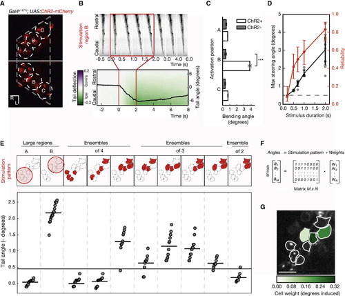
Functional Identification of Behaviorally Relevant Neurons (A) Probing the neuronal substrates driving a motor outcome. Slightly overlapping photostimulation regions, 18 μm in diameter, were targeted in fish expressing ChR2-mCherry in the nMLF for an initial characterization of the circuit. (B) Kinematics of the induced tail bending. When position B is targeted, a slow ipsilateral deflection of the tail is detected, followed by relaxation to the baseline level at the end of stimulation. The angle between the base and the caudal tip of the tail is shown as a black line, overlaid onto a heatmap, which shows the relative lateral deflection along the tail. (C) Comparison of the maximum tail bending angle induced by 2P photostimulation of different regions. The difference in deflection angle is only significant for region B (p value < 0.001; Welsh’s t test; Bonferroni corrected; n = 15 trials across six fish for ChR2+; n = 12 trials across four fish for ChR2−). Error bars indicate SEM. (D) The influence of photostimulation duration on behavior. Stimulations longer than 200 ms lead to tail deflection (judged as a deflection angle greater than five SDs of the baseline). Increasing the duration of the photostimulations causes tail bending in a larger fraction of trials (red) and larger amplitude tail deflections (black). Error bars indicate the SD. (E) Behavior-based identification of neurons driving tail bends. From the regions used for initial mapping, smaller subsets of neurons are iteratively selected for stimulation, based on the induced behavior magnitude (tail angle). This procedure, reducing trial after trial the number of units probed, converges to minimal selections of neurons that significantly drive behavior (at least five SDs above baseline—black horizontal line). (F) Model for neuron contribution to behavior. The magnitude of the tail angle (angles) induced in every trial is expressed as linear combination of the neurons included in the pattern (0, excluded; 1, included) and the contribution/weight of each neuron (weights). (G) Weight map of behavior. A regularized regression on the model in (F) is used to fit the behavior data. This returns a map with the contribution in degrees from each stimulated cell to the behavioral outcome. The scale bars represent 10 μm. |
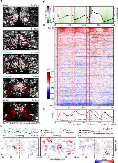
Combining Photostimulation with Functional Imaging and Behavior Recording (A) Multiplane recording of the activity of 486 cells during optogenetically induced behavior. Planes imaged in the midbrain of fish expressing ChR2-mcherry (red) and nlsGCaMP6s (gray) are shown. ROIs, corresponding to the cell bodies selected for analysis, are highlighted in white, and units selected for photostimulation are shown in cyan. (B) Kinematics of the tail in response to stimulation. This example shows the temporal evolution of the tail angle for four repetitions of 2-s photostimulation (red lines indicate stimulation onset and offset). Note that, at the third photostimulation episode, after an initial bending of the tail toward the side of the stimulation, the fish responded with a large-amplitude swim. Trials with this kind of transition bending-swimming were common in all the larvae tested (n = 3) and occurred in approximately 20% of the trials. (C) Raster plot showing the activity for the recorded neuronal population, with the same timescale as the behavior shown in (B). A small subset of neurons shows a reliable activity pattern temporally locked to stimulation and tail bending. A larger number of neurons show an activity increase corresponding to the large-amplitude swim. (D) Representation of temporal patterns in population activity by ICA. The first three components of the representation are shown: IC1 is associated to the activity during tail bending; IC2 represents the activity picked during the large-amplitude swimming bout; and IC3 represents a slow modulation in the activity not linked to a detectable behavior. (E) Circuit activity maps for the plane at z = 16 μm, showing the spatial distribution across the population of the three activity components. Representative traces, corresponding to the different ICs, are shown for the cells indicated with arrowheads in the corresponding maps (blue trace represents a stimulated cell). For IC2 and IC3, the calculated laterality indices were −0.13 ± 0.11 and 0.06 ± 0.15 (mean ± SD; p value 0.12 and 0.22), indicating slight, if any, ipsilateral bias. IC1, on the other hand, is significantly lateralized (−0.36 ± 0.15; p value 0.01). The scale bars represent 10 μm. |
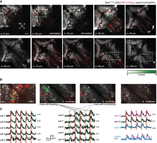
Imaging the Activity Associated with Behavior in Distant Brain Regions (A) Brain activity induced by nMLF activation. Activity across a large volume of the brain is captured by sequentially imaging ten planes, each separated by 12 μm (at four frames per second). Remote focusing of the imaging plane is combined with the 3D control of the photostimulation pattern to acquire GCaMP signals at each plane while keeping the stimulation targeted on the behaviorally identified neurons in the nMLF. Pixelwise regression analysis of the temporal series is used to pinpoint brain regions with activity profiles matching the stimulation epochs. For stimulation trials resulting in tail bending, the corresponding t-statistic for each pixel is averaged to create a map showing hotspots with activity associated with the behavioral outcome induced (in green). Also shown: ChR2-mcherry expression (in red), and nlsGCaMP6s expression (in gray). The scale bar represents 50 μm. (B) Higher-magnification view of the regions with dashed outlines in (A), focusing on areas with a high average t-statistic. In the plane at the level of the nMLF (z = 12 μm), where stimulation occurs, the activity is strongly lateralized. However, in the more dorsal layers, regions on both sides of the rostral and caudal hindbrain are active during tail bending. For the plane z = 96 μm, two maps are generated for the t-statistics: one considering trials with tail bending events and the other only trials with no behavior. The scale bar represents 10 μm. (C) Single-cell profiles of the induced activity in the hindbrain. Example ΔF/F traces (black), from selected neurons in (B), are shown along with the fit (green) and the corresponding coefficient of determination (R2) from the regression analysis. Red solid bars indicate trials that resulted in behavior, whereas trials without behavior outcome are indicated with dashed red bars. Two response profiles are shown (magenta and cyan; in detail on the right side), which have a noticeable difference in the timing of their responses. |
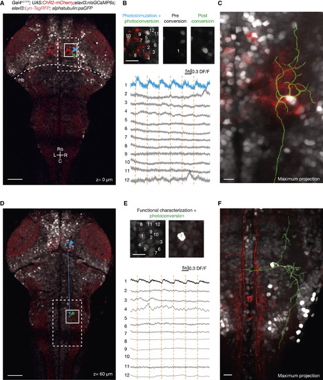
Morphological Reconstruction of Functionally Identified Neurons with Photoactivatable GFP (A) Combined ChR2 photostimulation, GCaMP imaging, and paGFP photoconversion. A larval brain with pan-neuronal expression of nlsGCaMP6s (gray) and Lyn-TagRFP (light red), ubiquitous expression of paGFP, and cells in the nMLF expressing ChR2 (bright red) are shown. The scale bar represents 50 μm. (B) Photostimulation + photoactivation protocol. First, a neuron is targeted for ChR2 photostimulation at 920 nm (cell 1; blue) while nlsGCaMP6s signals are imaged at 1,020 nm. The targeted neuron responds reliably to the stimulation. Such triggered activity is not detected in surrounding neurons. Afterward, the same photostimulated neuron is targeted for 2P paGFP photoactivation with 1 s of 750-nm illumination, resulting in a strong increase in fluorescence. Image extents are outlined in (A) in white. (C) Reconstruction of the targeted cell. After the diffusion of paGFP, the cell is imaged and its basic morphology can be traced. Image sizes are outlined in (A) with a dashed white box. (D) Morphological characterization of downstream neurons in the fish hindbrain recruited during nMLF photostimulation. As shown in Figure 6, activation of nMLF neurons drives activity in hindbrain neurons located 250–300 μm caudally. The scale bar represents 50 μm. (E) From a group of neurons in the hindbrain, imaged during nMLF stimulation, a secondary activated cell is identified and can be photolabeled with paGFP. Image sizes are outlined in (D) in white. (F) After applying the paGFP photolabeling protocol, functionally identified downstream neurons can be traced to reveal their morphology. Image sizes are outlined in (D) in dashed white. The scale bars in (B), (C), (E), and (F) represent 10 μm. Hb, hindbrain; Mb, midbrain. |
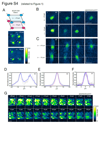
paGFP photoactivation (related to Figure 1). (A) Fluorescence signal measured in a zebrafish larva with pan-neuronal expression of paGFP after photoactivation with the 3D pattern shown in Figure 1C. The pattern consists of 7 illumination circles, 6 μm in diameter, placed at the corners of a 20x20x20 μm3 cube in the optic tectum. One corner was not illuminated to provide a comparison. (B) XY view of the fluorescent stack of the corresponding planes. Note that no fluorescence is detected from the plane at -10 μm in the region corresponding to the non-illuminated corner. (C) A side (XZ) view of the fluorescent signal. No fluorescence is detected in the region around -10 μm corresponding to the non-illuminated corner. (D) Intensity profiles in the XZ view from C. The two photoconverted foci, although with some extended and overlapping tails, are clearly separated and distinguishable. In blue is the average (3 measurements). (E) For comparison, we photoconverted paGFP with a single circle, 6 μm in diameter. Individual intensity profiles in the XZ view are shown in grey. In blue is the average across 4 photoconverted spots. The resulting FWHM measured along the z-axis is 8.9 ± 0.9 μm. In magenta is the average of the profiles recorded from a thin fluorescein layer. The photoconversion tails in the paGFP Z profile measured in vivo, can be explained by light scattering in the tissue (as reported in Hernandez et al., 2016). (F) XY intensity profiles from dataset in E (average in blue, fluorescein reference in magenta). The FWHM is 5.79 ± 0.91 μm, (G) paGFP expression coverage. A 20x20x20 μm3 cube is photoconverted by raster scanning the imaging beam at 750 nm. The stack acquired at 920 nm shows that, although with different expression levels, the majority of the cells are expressing paGFP. It is possible however to find cells without detectable paGFP photoconversion (<7.5% ± 2.2%, across different planes). This could be due to cells where the promoter is not active. |
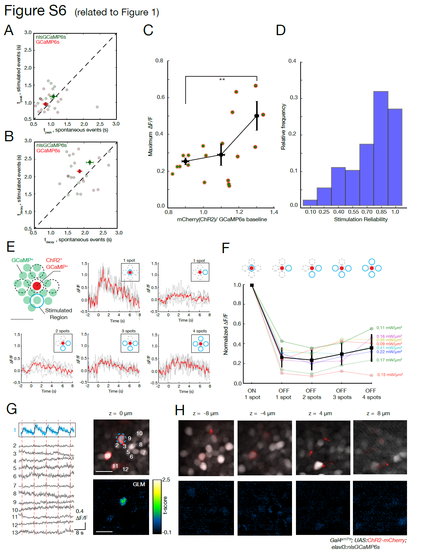
Characterization of induced GCaMP responses and photostimulation resolution (related to Figure 1). (A) GCaMP onset temporal dynamics. Comparison of the time to the peak (0 to 100%) for GCaMP responses imaged at 1020 nm for events driven by ChR2 photostimulation at 920 nm (0.1 - 0.22 mW/μm2) versus spontaneous events in the same cells. No significant difference was found between the stimulated and spontaneous conditions (p-value 0.35, t-test, saturated colors indicate means, with bars indicating s.e.m.) for GCaMP6s or nlsGCaMP6s. (B) Comparison of the decay time (to reach 50%) for the same molecules shown in A. No significant difference was found between the two conditions (p-value 0.16, t-test). (C) Dependency of the recorded ΔF/F on ChR2 expression level. Neurons expressing both nlsGCaMP6s and ChR2 were imaged at 1020 nm with 9 mW while being photo-stimulated at 920 nm with 0.11 mW/μm2. The maximum recorded amplitudes are plotted as function of the ratio between the fluorescence level of ChR2-mcherry and GCaMP baseline. Data were grouped into three bins, black dots and error bars indicate averages and s.e.m respectively (p-value 0.021, t-test). (D) Histogram of stimulation reliability. Individual cells were repeatedly stimulated, with many cells responding reliably. (50 trials from 10 cells). (E) Induced ΔF/F in neurons with off-target stimulations. These experiments validate the spatial selectivity of stimulation, starting with a reference using the response to a stimulation spot targeted exactly to a neuron expressing ChR2 (“on-target”, shown in red). This is compared to the response when one or more off-target spots are simultaneously stimulated, each 10 μm from the on-target cell. In all the trials, the power density per spot was constant and matched the power of the on-target spot. For each stimulation pattern (inset with blue icons), a 200 ms activation pulse was applied. The response of the on-target cell is shown in light grey for each trial, with the average in red (4 or more trials per stimulation pattern). (F) Response characteristics. With respect to the on-target stimulation, the normalized responses to off-target stimulations do not reach comparable levels of activity. The response characteristics for 8 cells (from 3 fish) are color coded, and in black is the mean value (error bars show standard deviation). The corresponding photostimulation power density per spot is indicated on the right. (G) Example of stimulation precision. A neuron expressing ChR2 is targeted with a 6 μm photostimulation spot. Simultaneous multiplane imaging provides the activity of neurons in the same and nearby planes. On the left are ΔF/F traces for target cell (blue) and surrounding cells. The position of the recorded cells is shown in the upper right panel. The lower right panel shows the t-scores from a pixel-wise generalized linear model (GLM, details in STAR Methods). The targeted cell has the highest tscores for this model of activity based on the stimulation protocol. (H) Other neurons show only low t-scores, indicating they are not effectively activated by the stimulation. Scale bar is 10 μm. |
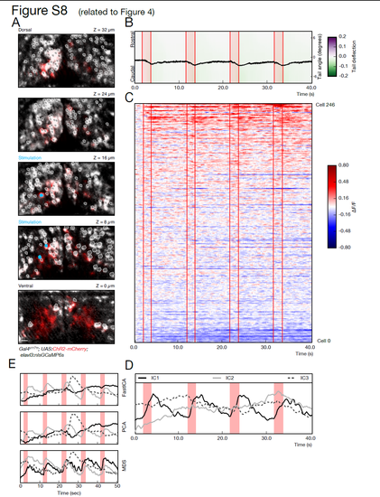
Investigation protocol demonstrated in an additional larva (related to Figure 4). (A) Volumetric recording of the activity of hundreds of neurons during stimulation-induced behavior. 5 planes are imaged in the midbrain of a fish expressing ChR2-mcherry (red) and nlsGCaMP6s (grey). ROIs corresponding to the cell bodies selected for the analysis are highlighted in white, and neurons selected for the photostimulation are shown in cyan. (B) The kinematics of the tail show a reliable tail deflection upon stimulation (red lines indicate stimulation onset and offset). (C) Raster plot showing the activity for the recorded population of 246 neurons, temporally aligned with the behavior recording shown in B. Similar to the example in Figure 4, a small subset of neurons shows a reliable activity pattern temporally locked to the stimulation and tail deflection. (D) Representation of common patterns in population activity by independent component analysis. The first component captures the stimulation induced network activity that corresponds to the tail bending behavior. (E) Comparison of dimensionality reduction methods on the same data shown in Figure 4. The different methods tested, Independent Component Analysis (fastICA), Principal Component Analysis (PCA), and Multi-Dimensional Scaling (MDS), all capture a rather similar representation of the network. One component captures the consistent activity induced by photostimulation, and a different component picks the activity associated with the large swim. The ICA and PCA representations are almost identical, while for MDS, which is a non-linear a manifold learning technique, the activity induced by stimulation is partially distributed into two components. Scale bar is 10 μm. |
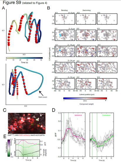
Dimensionality reduction representation of circuit dynamics (related to Figure 4) (A) The network activity of 486 neurons is projected into a simplified three dimensional space obtained by independent component analysis. The color encodes the temporal evolution of the network state, with stimulation phases indicated by red arrows. Each stimulation epoch shifts the circuit into a different state, with a return towards baseline following the end of stimulation. In this compact representation, the trajectory of the network activities associated with tail bending are well separated from the large swim bout. (B) Spatial patterns of the independent components at each imaged plane. The relative weights of neurons in the independent component representation are used to visualize the spatial organization of these common activity modes across the circuit. IC1, capturing the dynamics temporally locked to tail bending, shows a focused and lateralized pattern near the stimulation site. IC2 (swimming) and IC3 (slow circuit dynamics), have a broader and more symmetric distribution of activity across the midline. (C) Induced network activity resulting from nMLF stimulation driving behavior. Stimulated neurons are marked with a blue arrow. Scale bar is 10 μm. (D) Two different activity patterns in the circuit associated with the tail deflection can be detected, when comparing the neuronal responses ipsilateral versus contralateral to the stimulation side (light pink and green squares in C respectively). While in cells ipsilateral to the stimulation an increase in activity is detected (grey lines for single trials, pink trace for mean), a signal decrease in some of the contralateral neurons is noticeable (green trace for mean). (E) The activity profile recorded on the contralateral side (green trace), although temporally synchronized to the stimulation and tail deflection, shows a distinct temporal shift (see main text for quantification). |