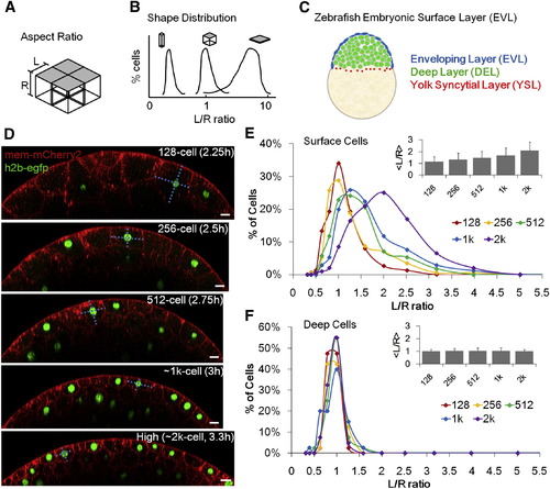
Quantitative Description of Surface Cell Shape Change of Zebrafish Embryos

(A) Schematic illustration of simplified epithelial monolayer, gray indicates the free surface, cell shape is represented by aspect ratio L/R.

(B) The morphology of an epithelial layer is represented as a distribution of L/R ratios.

(C) Zebrafish enveloping layer (EVL, blue) in the context of the whole embryo. Sketch represents a lateral cross-section of an oblong (~4 k cell) stage embryo.

(D) Time-lapse imaging data and measurement of surface cell L/R ratios (dashed cyan lines). Scale bars represent 20 µm. See also Figures S1D–S1H.

(E) Morphogenesis of surface layer over five cell cycles. n = 860. Inset: average L/R ± SD.

(F) Morphogenesis of deep layer over five cell cycles. n = 200. Inset: average L/R ± SD. The variance of ln(L/R) of deep cells is smaller than that of surface cells (f tests).

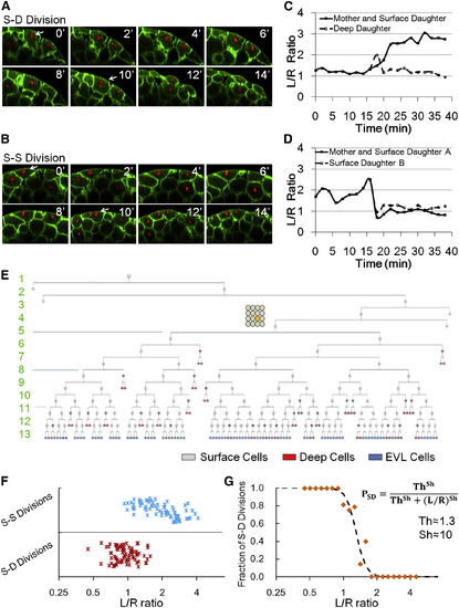
Division Patterns Determine N_S, and Cell Shape Is Predictive of Division Orientation

(A and B) Time courses of example S-D (A) and S-S (B) divisions. Arrows indicate the tracked cells.

(C and D) Example S-D (C) and S-S (D) mother and daughter L/R dynamics throughout the cell cycle.

(E) Full lineage up to 13^th cell division of a middle blastomere at 16 cell stage (highlighted yellow cycle). For simplicity, deep cell branches are not drawn as the subsequent divisions always make more deep cells. Numbers indicate cell cycle number.

(F) Relationship between cell shape and division choice. Each marker represents a tracked cell. n = 162. See also Figures S3A and S3B.

(G) Fraction of S-D division calculated by binning data in (F) according to L/R values. A Hill function switch is used to fit data points.

Mechanical Regulations on the Cell Shape Distributions

(A) A log-normal model fit of the cell shape distribution data (512 cell stage from Figure 1E, log-normal model p = 0.16, normal model (rejected): p = 2.7 × 10⁴, Χ² tests). See also Figure S4A and Data S1, Text 6 for other time points and statistics.

(B) Cell shape distributions represented by two parameters under the log-normal assumption. The differences between pairs of µ are significant (t tests) and the differences between pairs of σ are not significant (f tests).

(C) Cell shape changes after mitosis. Images show a group of surface cells changing surface areas following division (green, cell membrane; red, cell nuclei). Asterisks indicate S-D dividing cells in cytokinesis. Arrows show a S-S daughter expanding boundaries into a S-D daughter thus reducing their initial differences in L/R after divisions. Plot shows the shape distribution changes following division. Inset: corresponding <L/R> values (not significantly different, t tests on ln(L/R)).

(D) Schematic illustrations of surface configurations with high/low cortical tension and respective transition point angles (θ). The stronger the cortical tension the smaller the value of θ. See also Figure S4D and Data S1, Text 7.

(E) Cartoon illustration of mechanical interactions changing cell shapes. The five cells have variable shapes after division then evolve to reduce surface energy while meeting the constraints of constant total surface area and cell volume. Unfavorable shapes such as very columnar and squamous cells (corresponding to low and high L/R values) are reduced.

(F) Surface Evolver modeling of the change of shape distribution after division (512 cell stage). The images show the surface view of the cells, and the R dimension is perpendicular to the image plane (equivalent of a top view on the images in [E]). The configurations arrive at a near-stable state after approximately six iterations. See also Movie S3 and Data S1, Text 8.

(G) Evolution of L/R distributions. The log-normal model uses calculated µ and σ from simulated data at iteration 98 (stable state). Iterations 1–4 fit log-normal (Χ² tests).

(H) Effect of γ on L/R distribution change. Note the overlap between solid lines (iteration 10) from smaller γs and dashed lines (iteration 3) from larger γs. See also Data S1, Text 8.

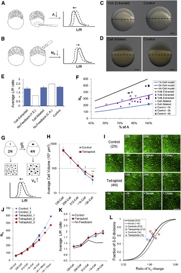
Robustness of Morphogenesis to Geometrical Parameters

(A, B, and G) Schematic illustration of perturbation methods on A (yolk extraction), N_S (cell ablation), V_C (tetraploid induction), respectively. The plot shows the predicted immediate change of cell shape distribution following perturbation. See also Figures S6A–S6C and Data S1, Texts 12 and 13.

(C and D) Phenotypes of yolk extraction (5 hr postfertilization [hpf], perturbed at 256 cell stage) and cell ablation (3.3 hpf, perturbed at 128 cell stage). The perturbed embryo in (C) has a smaller yolk (92% in diameter) and has an 85% smaller A; the perturbed embryo in (D) has the same yolk diameter but has a smaller total cell volume (<80%). Scale bars represent 100 µm. See also Figure S6D.

(E) <L/R> values after perturbations. Error bars indicate SEM. Dashed line bars are model predictions for corresponding perturbations assuming no feedback. See also Data S1, Text 12.

(F) Scaling of A and N_S in single embryos. Each mark represents one embryo. Lines show interplay model predictions. See also Data S1, Text 12.

(H) Surface cell volumes of control and tetraploid embryos over different cell-cycle stages. The absolute timing is different between controls and tetraploids as tetraploid cells slow down cell cycles earlier (Figure S6G). Volumes are measured using L²R. Error bars indicate SD. p = 6.8 × 10⁴, p = 5.4× 10⁵. The p values for the other three points are >0.1 (t tests).

(I) Surfaces of control and tetraploid cells indicating the density of surface cells. Images are 3D-maximum projections from a center-top view on the surface. The difference is subtle by 1 k cell stage and is more apparent at later stages. Scale bar represents 100 µm.

(J) N_S counts of control and tetraploid over time.

(K) <L/R> of control and tetraploid surface cells over time. Error bars indicate SEM. The No-feedback model prediction assumes no S-D division ratio change in tetraploid embryos despite V_C increase. See also Data S1, Text 13.

(L) Change of S-D division ratio as predicted by model and measured in controls and tetraploids. See also Data S1, Text 13.

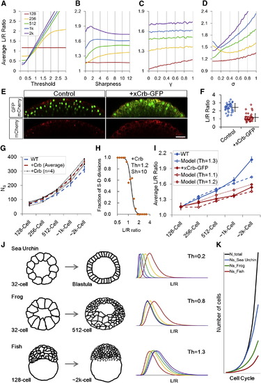
Effect of Model Parameters on Epithelial Morphogenesis

(A–D) Interplay model simulations of <L/R> using one variable parameter while fixing other parameters as in Figure 5C.

(E) Crb and control phenotypes at sphere stage. xCrb-GFP is visible as diffuse GFP signal in the image. Embryos are transgenic for H2B-GFP and mem-mCherry2. Scale bar represents 50 µm.

(F) L/R ratio measurements for embryos in (E). Error bars are SD.

(G) N_S trends in Crb embryos. The wild-type (WT) data is from Figure S2H. At ~2 k cell stage, two Crb+ data points are larger than 2× SD of the WT and two are larger than 1× SD (p = 0.002). Error bars are SD.

(H) Division rule in Crb injected cells. n = 122. In mother cells that satisfy 1 < L/R < 1.3, SS:SD for Crb+ cells is 17:27 (due to oblique divisions) whereas for WT is 11:39. See also Figures S7E and S7G.

(I) Interplay model prediction of Crb+ dynamics. For simplicity, the only changed parameter compared to WT simulation is Th, despite observations that A, γ also changed slightly in Crb+ embryos. WT data is from Figure 1E. n = 400 for Crb+ data from four movies. Error bars are SEM.

(J) Simulation of sea urchin (Wray 1997) and frog (Chalmers et al., 2003) embryo surface morphogenesis using an altered Th value and different initial conditions (A₁,V_C1,N_S1) and compared to fish. See also Data S1, Text 14.

(K) N_S changes of different species as a result of Th differences. The same Th values as (J) were used. See also Figures S7I and S7J and Data S1, Text 14.

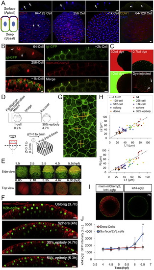
Epithelial Properties of the Pre-EVL Surface Layer and Imaging, Related to Figure 1

(A) Junction and polarity analysis of the surface cells. The schematic illustration shows two adjacent surface cells. Red indicates tight junctions as shown in ZO-1 staining images on the right; yellow indicates adherens junctions as shown by E-cadherin (CDH1) staining; green corresponds to the basal-lateral marker lgl as shown in (B); purple indicates aPKC (Fukazawa et al., 2010 and Krens et al., 2011). Arrows indicate focused staining signals. Scale bars: 20µm.

(B) Live imaging of embryos injected with lgl-GFP (Chalmers et al., 2005) mRNA. The GFP signal is detectable by 64-cell stage albeit being quite weak. GFP is detected on the basal lateral surface but not the apical surface. Scale bars: 10µm.

(C) Diffusion barrier function of the surface layer (pre-EVL). Embryos (128,256-Cell stages) were soaked in fluorescent dyes of different sizes and imaged for <20 min. No dye signal was detectable under the surface layer even when the exterior imaging signal is saturated. As a positive control the 10kd dye was injected into the embryo. Dye signal was found between cells (arrows) and stayed (at least 20 min). Embryos are transgenic for h2b-EGFP and mem-mCherry2.

(D) Schematic illustration of imaging timeline and protocol, including imaging set-up and spatial-temporal coverage and resolution. Embryo illustrations courtesy of Kimmel et al. (1995). See also Extended Experimental Procedures.

(E) Example time courses focusing on a lateral view and a top view, respectively. Fluorescent proteins labeling the membrane and the nucleus of cells were used. Lateral view: mem-EYFP and h2b-tomato; top view: mem-mCherry and h2b-EGFP. The lateral view images were generated using a data set partially published in Xu et al. (2012).

(F) Extended timelapse imaging data following Figure 1D. Scale bars: 20µm.

(G) Error analysis of L/R simplification in zebrafish surface cells. The image (3D maximum projection) illustrates free cell surfaces from a top view. The measurement of L in cross-sections (Figures 1D and S1F) brings an error as a difference between L1 and L2 exists.

(H) Comparison of L1/L2 and L1/R at different stages in surface cells. The L1/R difference is 13.5% ± 14.3% while L1/L2 difference is 0.5% ± 11.4%. n = 51. This indicates that using either L1 or L2 for calculating < L/R > is equivalent. The difference between L1 and L2 has a standard deviation of <11% which introduces a small amount of variability in L/R values that affects the accuracy of reported L/R distribution. See discussion in Data S1, Text 2.

(I) tg(krt4:egfp-caax) EGFP expression in differentiated EVL cells (Krens et al., 2011).

(J) Time course of tg(krt4:egfp-caax) EGFP intensity in surface cells and deep cells. n = <70 cells per time point measured. At 5.5h p = 0.08; p = 5e-6; p = 1e-14 (t tests).

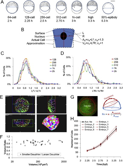
Measurements and Distributions of Surface Area, Cell Volume, and Cell Number, Related to Figure 2

(A) Schematic illustration of macroscopic surface area and volume measurement using whole embryo lateral images. Both illustrations and actual photographs (not shown) are used. The image is fit with a circle to approach the surface shape and a chord is drawn on the vegetal edge of surface cells. The surface area and volume of the resulting spherical cap provides rough whole embryo estimate values of A and V_C. Embryo illustrations courtesy of Kimmel et al. (1995). See also Data S1, Text 3.

(B) Schematic of microscopic estimation of A_C and V_C. See also Data S1, Text 3.

(C) Distribution of normalized L². The distribution fits a log-normal model.

(D) Distribution of normalized L²R. The distribution fits a log-normal model.

(E) Examples of full membrane segmentation to measure V_C using ACME and GoFigure 2. See also Movie S2 and Extended Experimental Procedures.

(F) Ratio of sister cell volumes (smaller/larger). Data points used full membrane segmentation measurements as in (E). 7.3% ± 5.2% difference from average V_C of two daughters, n = 43 pairs.

(G) Schematic illustration of surface cell counting method. Due to the spherical curvature and imaging limitations only partial surfaces were acquired, and thus an estimation of N_S was made by drawing a circle on 3D perspective views of the surface. The total number equals the cell number in the circle multiplied by the ratio between surface area of the circled cap and the whole surface.

(H) Individual N_S counts of 7 embryos and average. The average values were used in Figure 2 and following modeling work. “Embryo_7” is counted from a movie by Keller et al. (2010).

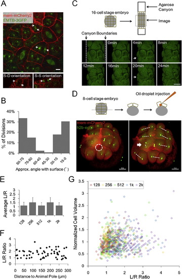
Division Orientations and Geometry Models of Cell Shape Distribution, Related to Figure 3

(A) Centrioles and spindles highlighted by tg(actb2:EMTB-3GFP) embryos (Wühr et al., 2010). Arrows: centrioles. Scale Bar: 10µm.

(B) Division orientation angle distribution. n = 128. Angles between the straight line through anaphase daughter nuclei and the surface are measured.

(C) Changed division orientation by squishing. Dashed lines showing the agarose canyon walls pressing on the edge cells of a 16-cell stage embryo. The blastomere (Arrow) becomes flattened and divided twice along the canyon wall, while it normally divides perpendicularly at the 2nd division. Scale Bars: 100µm.

(D) Changed division orientation by oil drop injection. Dashed white circle highlights the injected oil drop inside one of the 8 early blastomeres. This blastomere (Arrow) bulges at the top surface. Consequentially it divides perpendicularly to the surface generating an aberrant S-D division. Dashed lines highlight division orientation. Scale Bars: 100µm.

(E) Morphogenesis predicted by a pure geometry-division model (no mechanical coupling), applying the division rule Th = 1.3 and using 128-cell stage cell shape distribution as initial input. The result is oscillating < L/R > instead of observed gradual flattening.

(F) Spatial distribution of shapes. Cells were randomly sampled from different distances of the animal pole (projected distance ignores the surface curvature). Cells of different L/R ratios are found at different locations therefore spatially correlated heterogeneity of shapes is unlikely underlying the shape distribution.

(G) Correlation between V_C and L/R at all time points. V_C does not predict L/R ratio of the cell therefore the volume distribution is unlikely underlying the shape distribution.

Mechanical Modeling of Cell Shape Distributions, Related to Figure 4

(A) Log-normal fit of data (from Figure 1E) as in Figure 4A. See also Data S1, Text 6.

(B) Predicted S-D division ratio using log-normal fit in (A) and the division rule (Figure 3G).

(C) Predicted L/R distribution using log-normal fit and the division rule. A 2-peak distribution follows when cell shape changes after divisions are not considered.

(D) Local forces that mediate cell shapes. F_CM: cell-medium surface tension, F_CC: cell-cell surface tension, F_A: adhesion force, θ: transition point angle (Maître et al., 2012). See also Data S1, Text 7.

(E) Dissociated cells in Ca²⁺ free medium round up as spheres under cortical tension; adding Ca²⁺ allows them to recover adhesion to attach to dish bottom or other cells and deform from sphere.

(F) θ changes during the cell cycle in surface cells. Arrows indicate a decreased θ during and immediately after mitosis.

(G) γ as a function of time. γ values are calculated averages from measured θs of a cohort of tracked surface cells. θ is highly variable between different cells during divisions. Red arrows indicate the approximate time of cell divisions; the left-most arrow is the 2 to 4 cell division. Blue marks indicate the time points at which cell shape distributions were measured.

(H) Nocodazole treated embryos (8-cell stage treatment). The Nocodazole treated cells become more deformable. The treatment also stops cell cycles. Scale bar: 100µm.

(I) Cell shape distributions at 256-cell stage. Inset: < L/R > values (not significantly different, p = 0.38, t test on log(L/R)). σ is different (treated: 0.40, control: 0.32, p = 0.02, f-test).

(J) Surface cell morphologies at ~2k-cell+1h (green signal from mem-EYFP). Top images are 3D rendered views showing rounded edges of cdh1 MO injected cells, bottom images are cross-sections showing decreased θ (and γ). Scale bar: 30µm.

(K) Reduced flattening of cdh1 MO injected embryos in later stages by <10%. n = 60 cells from 3 embryos at each time point were measured for both groups. Error bars are SD. At ~2k-cell p = 0.096; p = 0.029; p = 0.011 (t tests on log(L/R)). σ is not different between control and MO groups (f-tests on log(L/R)).

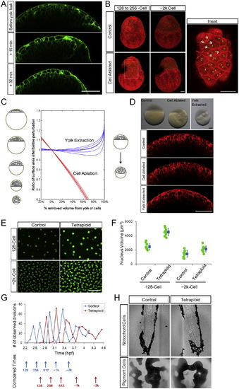
Phenotypes of Yolk Extraction, Cell Ablation, and Tetraploidy, Related to Figure 6

(A) Surface morphological changes following yolk loss. Embryos are fragile after yolk extraction procedure and are not suitable for immediate imaging mounting procedures. Here we found an embryo that had a yolk leak during live imaging. Green fluorescence marks cell membranes. All scale bars: 100µm.

(B) Local stretching and S-S divisions at the cell ablation site. Images are 3D maximum projections of H2B-EGFP, mem-mCherry labeled embryos. The dark region in the perturbed embryo shows the ablation site. Note that by 2k-cell stage the site has completely healed, however due to remaining debris at the ablation site its imaging signal is weak. Arrows: daughter nuclei of S-S divisions of surface cells that stretched toward the ablation site.

(C) Schematic (left) and theoretical (middle) effect of yolk extraction and cell ablation on total surface area of the surface cells. In reality, yolk extraction causes cells to bulge inward into the yolk (right) resulting further reduction of surface area. See also Data S1, Text 12.

(D) Phenotypes of yolk extraction and cell ablation. Embryos in upper bright field images correspond to confocal images below, showing similarly flattened surface cells. Red fluorescence indicates mem-mCherry.

(E) Nuclear sizes of control and tetraploid cells. Green fluorescence indicates H2B-EGFP.

(F) Quantification of nuclear sizes as in (D). Blue markers indicate average ± SD.

(G) Changed division time and cell cycle duration in tetraploid embryos. Division events are counted by the number of anaphase cells at each time point. The time points between divisions (marked by arrows) were chosen for V_C, N_S and < L/R > comparison in Figures 6H–6L.

(H) Verification of tetraploidy at later stage by sizes of differentiated cells in different tissues. Upper: notochord cells are larger and packed differently in tetraploids and blood cells are bigger. Lower: the skin pigment cells have larger surface area and visibly larger nuclei in tetraploids and are more clustered.

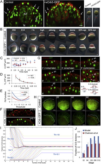
Effects of Parameter Changes on Morphogenesis and Steady States and the Effects of Crumbs Injection on Different Parameters, Related to Figure 7

(A) 30hpf EVL phenotypes of Crb3-GFP injected embryos. Images are cross-section confocal slices capturing the EVL/periderm (arrows), the neural tube (NT), the somites/muscles (S) and the notochord (N) at the indicated anterior-posterior level of the shown embryos (red bars in the bright field images on the right). The Crb3-GFP injected embryos have denser EVL cells that are more columnar shaped compared to controls (arrows) while other tissues appear normal. ~20% (18/94, 5 different experiments) of injected of embryos showing clear Crb phenotype at early stages (as seen in (B)) develop over 24hpf and appear shorter and delayed. Scale bar: 20µm.

(B) Time sequence of bright field lateral view images of Crb injected embryos. The embryos are not distinguishable in appearance compared to control (mem-mCherry injected) embryos in the pre-EVL stages. The difference arises at sphere stage where unlike controls that start to dome and spread, the Crb+ cells pull back (“reverse doming,” arrow). The phenotype becomes more apparent later (“reverse epiboly,” see also (H)) although 20% of these embryos do complete epiboly. Scale bar: 100 µm.

(C) Measurement of surface area of control and Crb injected embryos. Circles are global estimations, lines are N_S multiplying < A_C > as in Figure 2A. The change of shape of cells results in surface area changes that are more apparent in later stages.

(D) Cell volume measurement using < L²R >. The WT curve is from Figure 2B. No discernible difference of volume change rate is found in Crb+ embryos. Error bars are SD.

(E) Crb injected surface cells have a lower Th. Fit function is calculated by summing up the squares of differences between expected fraction of S-D division (predicted by Equation 17) and cell tracking data points. The smaller the fit function, the better the fit. For WT, data in Figure 3G is used; for +Crb, data in Figure 7H is used. For both Sh is set at 10.

(F) γ parameter is reduced in Crb injected cells. Arrows indicate less smooth surface at cell-cell contacts indicating an increased contact angle θ and smaller γ.

(G) Example instance of “oblique” divisions in Crb injected embryos. In oblique divisions (Chalmers et al., 2003), the division orientation is close to perfect S-D (perpendicular to surface), however, the presumptive deep daughter retains a small apical surface (d2 in the images) and remains a surface cell. This is a possible cellular mechanism of the observed effective Th change and the role of Crb in promoting apical membrane might explain the increase of oblique divisions. 16/122 of divisions tracked in Crb+ embryos were oblique, while rare occurrences were found in WT. Scale bar: 10µm.

(H) Retreat of epiboly frontier in Crb injected embryos. Images are 3D volume rendering of confocal stacks. The embryos are oriented sideways so the border between the cells and the yolk (the YSLs) can be followed. White lines mark the progress line (frontier) of epiboly using the edge of YSL nuclei. Red lines mark the frontier one hour later and progress of epiboly can be seen with the initial white lines. All of the Crb injected embryos exhibit “reverse epiboly.” Surprisingly, a fraction of these embryos (<20%) eventually return to progressive epiboly and develop into embryos as seen in (A). Scale bar: 100 µm. See also Movie S1.

(I) Convergence to steady states with similar S-D division ratios for most Th values between 0 and 1. See also Data S1, Text 16.

(J) Model prediction of S-D division ratio in frog and comparison with measurements by Chalmers et al. (2003) (data approximated from Figure 5B of this reference).