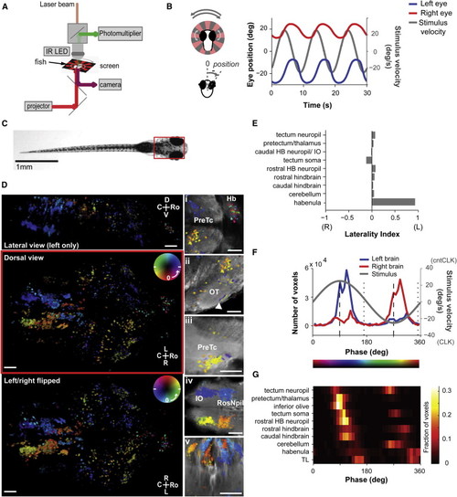
Imaging the Whole Brain of a Single Fish during Visuomotor Behavior

(A) Experimental setup. Zebrafish larvae were restrained in agarose, with their eyes and tail free, and placed on a screen for visual stimulation. Eye and tail movements were tracked while imaging brain activity with a two-photon microscope.

(B) Optokinetic response (OKR). Top left: larvae were presented with a rotating radial striped pattern. Bottom left: eye position was defined as the eye angle relative to the midline. Counterclockwise eye positions were defined to be positive. Right: larvae tracked the movement of the grating with a conjugate movement of the eyes. Stimulus rotation was sinusoidally modulated (gray, stimulus velocity). The mean eye position throughout the recording session is shown. In each imaging plane, the stimulus was presented three times. See also Figure S1 and Movie S1.

(C) Image of a 6-day-old larval zebrafish. Red box indicates the imaged area in (D). Scale bar, 1 mm.

(D) Activity phase maps show that different brain areas are modulated at different phases relative to the stimulus. Center left: rendered dorsal view of all ROIs in one fish, color-coded according to the phase of their response at the stimulus frequency (see Experimental Procedures and Figure S2); white marks in the color wheel show the peaks of stimulus velocity. Top left: lateral view of ROIs in the left half of the brain. Bottom left: dorsal view that has been left/right flipped, and the color map phase-shifted by 180 degrees, to illustrate the symmetry of responses in most brain regions. Right insets show zoomed-in views of ROIs overlaid on the average GCaMP5G fluorescence as an anatomical reference. (i)–(iv) are dorsal views, and (v) is a coronal view. (i) Habenula (Hb) and pretectum (PreTc). (ii) Cell somas in the optic tectum (OT) and layered responses in the neuropil (arrowhead). (iii) Pretectal retinal ganglion cell arborization areas. (iv) Inferior olive (IO) and rostral neuropil (RosNpil) in the hindbrain. (v) Cell columns in the hindbrain. Scale bars, 50 μm. See also Movie S3.

(E) Laterality index for different brain areas. The habenula showed marked asymmetry, with most activity occurring on the left side. HB, hindbrain; TL, torus longitudinalis.

(F) Distribution of phases of activation for voxels located in the left (blue) and right (red) halves of the brain. Phases are corrected to account for the delay introduced by GCaMP5G. Bottom color bar shows the correspondence between phase and map color.

(G) Timing of activation across brain areas. Normalized histogram of the phases of peak activity for different brain areas. Left and right areas have been pooled with a 180° phase shift. Phases are corrected as in (F).

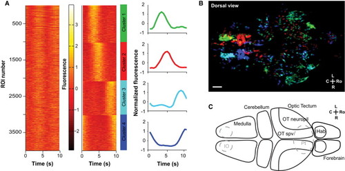
Clustering of Fluorescence Traces Reveals Four Temporal Clusters

(A) Activity traces of all ROIs can be grouped in four clusters. Left: activity for all ROIs of a fish (in rows); for each ROI, the normalized, average activity across all stimulus repetitions is shown. Center: ROIs sorted according to the cluster they fall into. Right: average of the Z score traces for each cluster. See also  Figure S3.

(B) Anatomical distribution of activity clusters in one fish. Sum projection showing the distribution of the four clusters of activity in the same fish as in (A), with colors corresponding to the color traces in (A). Scale bar, 50 μm.

(C) Schematic outlining relevant brain regions in the zebrafish larvae, in a dorsal view. OT, optic tectum; OT spv, optic tectum stratum periventriculare; IO, inferior olive; Pt, pretectal area; Hab, habenula. Gray dashed lines demarcate areas located more ventrally.

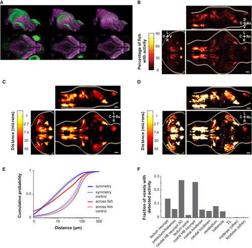
Morphing onto a Reference Brain Reveals Stereotypical Activity

(A) An individual larva brain (green) is morphed in three dimensions onto a reference brain (magenta) by performing an affine followed by a nonrigid alignment.

(B) Maximum projections from three orthogonal views, showing the percentage of fish (n = 13) imaged that show activity at each voxel (after registration) for all voxels within the brain. Scale bars in all panels, 50 μm.

(C) Minimum projections of the median distance that needs to be traveled in every other brain to find a similarly active voxel (see Experimental Procedures). The data are averaged across all comparisons (n = 13 fish, 156 comparisons).

(D) Minimum projections of the median distance that needs to be traveled to find a similarly active voxel in the left/right flipped of the same brain. The data were averaged across all fish (n = 13).

(E) The cumulative probability for finding a similarly active voxel within a given distance for the data in (C) (red) and (D) (blue). The data are averaged across all comparisons (red line, n = 13 fish, 156 comparisons). To control for the overall spatial distribution of ROIs, the same analysis was performed with the phases of the starting ROIs randomly shuffled (dotted lines).

(F) Fraction of detected active voxels by brain region in imaging data averaged across three individual brains from fish that were selected based on similarity of behavioral profile during imaging.

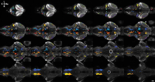
Averaging Raw Data from Morphed Brains Provides a Comprehensive Map of the Areas Active during Behavior

Color-coded activity phase of ROIs segmented from volumetric imaging data averaged across three fish. ROIs are superimposed on average GCaMP5G fluorescence for anatomical reference. Average planes are shown at 10 μm intervals from a stack of 510 image planes with 0.5 μm z-separation. Features highlighted are the oculomotor nucleus (solid line), the interpeduncular nucleus/median raphe (dashed line), the pretectum (arrowheads), and retinal ganglion cell arborization fields (arrows). See also Movies S6 and S7.

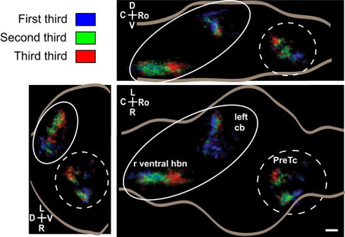
Spatial Gradients of Activity Timing Are Found in Various Brain Regions

Voxels were color-coded blue, green, or red depending on whether they fell into the first, second, or third third of voxels active within that region; that is, in each region, blue voxels were active before green voxels, which in turn were active before the red ones. A caudal-to-rostral gradient of activity timing is visible in the cerebellum (cb) and ventral hindbrain (r ventral hbn; only left cerebellum and contralateral hindbrain are shown for simplicity [solid line]), whereas a rostral-to-caudal gradient is observed in the pretectum/thalamus region (PreTc; only right is shown [dashed line]). Regions circled together were analyzed together; activity in the cerebellum (cb) and the contralateral inferior olive and more rostral neuropil show simultaneous activity. Only the cerebellum and pretectal region are displayed in the coronal projection for simplicity. Data are the average of three fish, as in Figure 4. See also Movie S8. Scale bar, 50 μm.

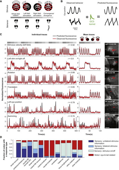
Sensory and Motor Signals Are Reflected in the Measured Activity

(A) Four stimuli were used to separate different sensorimotor signals: the standard rotating grating, rotating gratings presented on the left or right visual fields alone, and gratings rotating in opposite directions for each eye, to simulate forward and backward motion. Top: visual stimuli. Bottom: schematic of the behavior (eye rotation or tail movements) elicited. See also Figure S1B. Gray shades indicate the four stimuli periods.

(B) Behavioral and stimulus-related variables were convolved with an exponential kernel using the decay time constant of GCaMP5G (Chen et al., 2013b). These convolved traces represented the predicted fluorescence that would be recorded if activity was related to each of those variables (see Experimental Procedures and Miri et al., 2011b). See also Figure S4.

(C) ROI activity is strongly correlated with the predicted fluorescence for different behavioral variables (regressors). For each example ROI, the fluorescence trace and the predicted fluorescence for the regressor with the highest correlation are shown. Left: normalized (Z score) fluorescence traces for a subset of stimulus repetitions, and the corresponding normalized (Z score) behavioral trace. The correlation coefficient is indicated. Center: normalized average fluorescence across stimulus repeats (and planes) for the ROI, with the corresponding normalized average behavioral trace. A schematic of the four stimuli is shown above the top center plot. Gray boxes indicate the duration of each of the four stimuli in all plots. Right: anatomical localization of the ROIs (red). See also Figures S5 and S6. Scale bars, 50 μm.

(D) Sensory and motor variables are differentially represented in different brain areas. Fraction of cubes best correlated with different categories of regressors in different brain regions (best r > 0.3). Sensory variables were divided in three categories: one that included features related to stimulus motion, one that encompasses responses related to stimulus onset/offset, and another in which information was combined from the two eyes. Motor variables included those related to eye position or velocity and swimming.

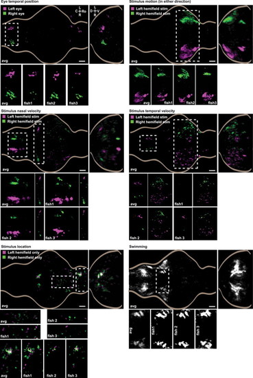
Consistent Localization of Sensorimotor Signals in the Zebrafish Brain

Distribution of cubes that correlate best with particular sensory and motor variables (r > 0.3) averaged across seven fish. The location of many correlation-defined regions in the maps shows remarkable consistency across fish. For each regressor/regressor pair, a z-sum projection and a coronal sum projection are shown. Coronal sections were smoothed along the z axis with a 1.5 μm Gaussian filter. For each map, an area of interest is highlighted in the whole-brain map and a detailed view of this area is shown for the average map, alongside the identical region, in three example fish. See also Figure S7. Scale bars in all panels, 50 μm.

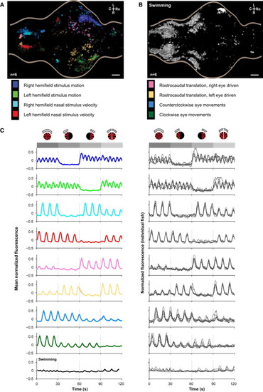
Functional Dissection of Activity Based on Multidimensional Clustering

(A) Rendered dorsal view of the anatomical distribution of four symmetrical functional clusters, averaged over seven fish, from k-means clustering of the behavioral correlation vectors of responsive cubes. See also Figure S8 and Movie S10.

(B) Rendered dorsal view of the combination of five symmetric clusters that show strong correlation with tail movement, averaged over seven fish.

(C) Fluorescence traces for each of the nine cube cluster groups shown in (A) and (B) for individual fish (right) and averaged across the seven fish (left; gray shading represents SEM). A schematic of the four stimuli is shown (see Figure 6 and Figure S1). Gray boxes and dotted lines indicate the duration of each of the four stimuli in all plots.

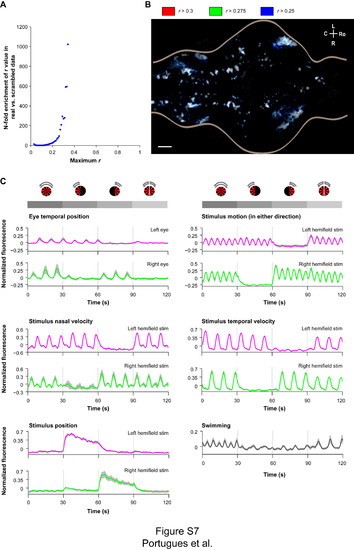
Threshold choice and traces for regressor maps (related to Figure 7)

(A) The N-fold enrichment of the maximum absolute regression coefficient (across all regressors) for every voxel in the real data compared to the equivalent computation performed using shuffled versions of the same regressors (8 second blocks; n=1,568,168 cube ROIs from 7 fish). The value of 0.3 is more than 200 times more common in the real data, indicating that this is a conservative threshold for selecting ROIs with activity correlated to the behavior.

(B) Z-projection of voxels with activity correlated to at least one regressor at three different thresholds: 0.25 in blue, 0.275 in green and 0.3 in red. The pattern of white areas with blue borders shows that reducing the threshold changes the boundaries of identified regions and contributes noise, but does not result in the identification of more active areas, and indicates that the map is robust to the precise choice of threshold. Scale bar is 50 microns.

(C) Average normalized fluorescence traces for the functional structures shown in Figure 7. All traces are the mean across fish with SEM shown by gray shading (n=6 fish). A schematic of the four stimuli is shown. Gray boxes and dotted lines indicate the duration of each of the four stimuli in all plots.

Clusters from Figure 8A (related to Figure 8)

We plot the eight clusters from Figure 8A in corresponding pairs for ease of viewing. Scale bars are 50 microns. Note that in the two upper panels, activity relates to stimulus motion in either the right or left hemifields, regardless of the stimulus on the opposite hemifield. In the left lower panel, on the other hand, activity in the two clusters results from integrating the stimuli in both hemifields. For instance, in the case of ′rostrocaudal translation, right eye driven′, activity occurs when the right hemifield is presented with nasal to temporal (rostrocaudal) motion, but is suppressed when the left hemifield is simultaneously presented with temporal to nasal motion (i.e. during rotational motion).