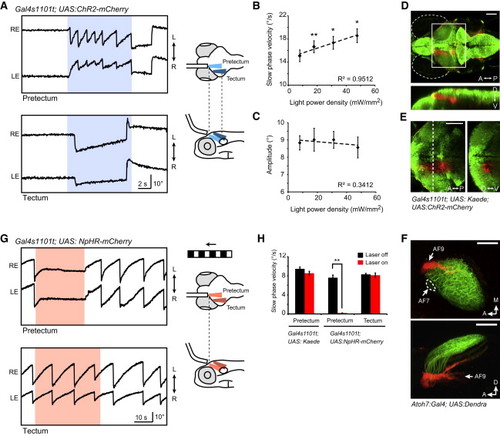
Optogenetic Manipulations of the Pretectal Area during OKR

(A) Angular eye position during ChR2 stimulation in the pretectal (top) and tectal (bottom) area. Blue-shaded regions depict the epoch of ChR2 stimulation (power density = <18 mW/mm²). Schematics of optical stimulation are shown on the right. An optic fiber (diameter 50 μm) was positioned in parallel to the fish’s longitudinal axis and angled ventrally. For tectum stimulation, the optic fiber was shifted laterally and posteriorly compared to the pretectum stimulation. LE indicates left eye; RE indicates right eye.

(B and C) Velocity and amplitude of slow-phase eye movements evoked by ChR2 stimulation as a function of laser power density. Right and left stimulations were pooled, and the eye contralateral to the stimulated side was measured (n = 6 fish). p < 0.01; p < 0.05; paired t test against the lowest laser power density. R² indicates square of Pearson’s correlation coefficient.

(D) Confocal z projection of a Gal4s1101t; UAS:ChR2-mCherry; UAS:Kaede fish in dorsal view (top) and side view (bottom). Kaede was locally photoconverted (red) in the left pretectum.

(E) Single optical section (3.6 μm) of the photoconverted area; corresponding to the white box in (D) in dorsal view (left). A frontal view at the level of dashed line is shown on the right.

(F) Photoconversion of RGC axons. Confocal z projection of an Atoh7:Gal4; UAS:Dendra larva after photoconversion using a 50 μm optic fiber in dorsal view (top panel) and side view (bottom panel). Photoconverted Dendra (red) was detected in AF9 and the deepest layer of the tectum (which receives projections from RGCs that project to AF9), whereas AF7 and most of the tectum (AF10) remained unconverted (green).

(G) Representative eye traces of an NpHR-stimulated animal during OKR. Red-shaded regions indicate the epoch of NpHR stimulation (633 nm; <140 mW/mm²). Schematics of visual and optical stimulations are shown on the right.

(H) Slow-phase velocity of the OKR under laser off and on conditions (n e 6 fish for each condition). The eye contralateral to the NpHR-stimulated side was measured. p = 0.00064, paired t test. A indicates anterior; P indicates posterior; D indicates dorsal; V indicates ventral; M indicates medial. Error bars indicate SEM. Scale bars show 100 μm (D–F).

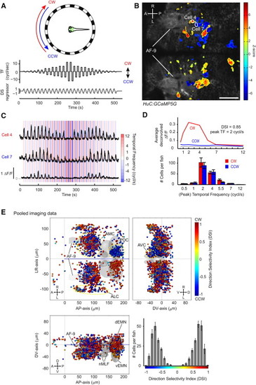
Calcium Imaging of the Pretectum Reveals High Degree of Direction Selectivity during Whole-Field Motion

(A) Illustration of the stimulus protocol for two-photon calcium imaging during simultaneous visual stimulation. (Top) An LED arena surrounding the fish was used for visual stimulation. The green box shows the approximate region imaged in (B). (Middle) Stimulus directions were alternated (CW or CCW) and had varying temporal frequencies (TF, 0.5–12 cycles/s). (Bottom) A direction-selective (DS) regressor was built from the stimulus protocol.

(B) 2D map of image pixels that are correlated with the DS regressor, superimposed on an optical section of the HuC:GCaMP5G transgenic animal. Pseudocolor scale shows the local correlation to the DS regressor (Z score, see Experimental Procedures for details). A: anterior; P: posterior; R: right; L: left.

(C) Fluorescence (ΔF/F) traces during the visual stimulus presentation. The cell numbers correspond to the ones in (B). Cell 4 responded during CW rotation, whereas cell 7 responded during CCW rotation. Both cells responded to temporal frequencies ranging from 0.5 to 7 cycles/s and less so to 12 cycles/s.

(D) (Top) Tuning curve of the cell plotted at the bottom of (C) during the CW (red) and CCW (blue) stimulations. The gray line indicates the threshold used for DSI calculation (see Experimental Procedures). (Bottom) Histogram showing the distribution of peak temporal frequencies per fish (n = 7 fish).

(E) 3D reconstructed map of CW- and CCW-responsive cells. Each dot represents a cell and is color-coded according to its direction selectivity index (DSI). Coordinates are defined as distances relative to the anterior-dorsal edge of neuropils in the diencephalon (anterior-posterior axis and dorso-ventral axis) and midline (left-right axis). dEMN indicates dorsal extraocular motor neurons; vEMN indicates ventral extraocular motor neurons; together, dEMN and vEMN correspond to the trochlear and oculomotor nuclei; nMLF indicates nucleus of the medial longitudinal fasciculus. Cells cluster in four anatomical regions (see Results): AMC, ALC, AVC, and PDC. (Lower right) Histogram of DSIs per fish (n = 7 fish). Error bars indicate SEM. Scale bar shows 50 μm. See also Figures S1–S4.

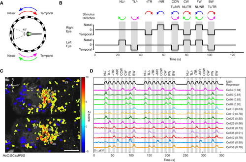
Calcium Imaging of HuC:GCaMP5G Fish in Response to Monocular and Binocular Stimulation

(A) Schematic diagram of the experimental setup. The fish’s central visual field (45°) was masked to avoid stimulation of the binocular visual field. The green box shows the approximate region imaged in (C). Each half of the LED arena was rotated in nasalward (N) or temporalward (T) direction.

(B) Visual stimulation protocol. NL/ indicates nasalward motion to left eye; TL/ indicates temporalward motion to left eye; /TR indicates temporalward motion to right eye; /NR indicates nasalward motion to right eye; CCW indicates counter-clockwise; CW indicates clockwise; FW indicates forward; BW indicates backward.

(C) Z score map of an example recording showing motion-correlated pixels colored in red/yellow. The main regressor used for analysis is shown in the top row of (D). A indicates anterior; P indicates posterior; R indicates right; L indicates left.

(D) Example fluorescence (ΔF/F) traces (colored lines) from the single recording in (C). The eight different stimulus phases (shown in gray vertical bars) were repeated three times in one recording. Cell numbers correspond to the labels in (C). The best-performing regressor traces (gray lines, see Results) are overlaid on ΔF/F traces. Correlation coefficients with the corresponding regressors are given in parentheses. Scale bar shows 50 μm.

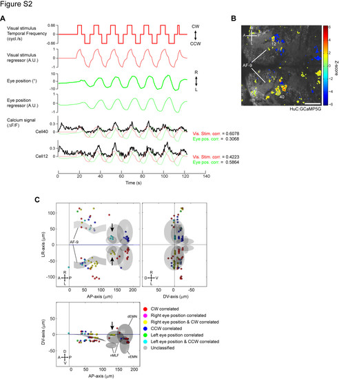
GCaMP imaging with simultaneous eye tracking in a non-paralyzed preparation (related to Figure 2).

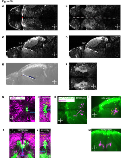
Registration procedure and landmarks (related to Figure 2).

(A, B) Dorsal view of a HuC:GCaMP5G larva. The xy-position of the origin (red asterisk) is defined by the intersection of a line connecting the anterior tips of the AF9 containing neuropil (A) and the midline (B). The dorsoventral position of the origin is defined by moving dorsally in the z-stack until the anterior tips of the AF9 containing neuropil are not visible anymore (A). (C, D) In sagittal view, lines are drawn along the dorsal border of the AF9 containing neuropil in the left (C) and right (D) hemispheres to measure the pitch angle of the animal relative to the imaging plane. (E) The precise position of the dorsal edge of the AF9 containing neuropil (blue points) and the origin (red asterisk) are overlaid on a projected sagittal view. In addition, the registration line from (C,D) is overlaid (white) to show that the course of the border of the neuropil at particular medio-lateral levels (C,D) does not capture the overall curvy shape that is evident when measuring the medio-lateral center points of the dorsal edge of the neuropil (blue points). (F) The schematic neuropil landmark (gray, z-projected) is overlaid on a single optical slice located 40 μm below the posterior commissure (dorsal view). Note that the schematic shape does not match the medio-lateral extent of the neuropil, since the schematic shape only corresponds to the dorsal border of the AF9 containing neuropil and the more dorsally located neuropil (see e.g. Figure S4B) is located further medially. (G-J) The dorsal extraocular motor neurons (dEMN) and ventral extraocular motor neurons (vEMN) were imaged in vglut:dsRed; isl1:GFP transgenic larvae. (G) Optical slice at the dorso-ventral center of the vEMN (dorsal view). (H-J) Dorsal, frontal and sagittal images were projected along the extent of dEMN and vEMN. Image volumes dorsal to the dashed line in (I) are projected in (H). (K-M) Projected images of one of the backfilled HuC:GCaMP5G larvae used for measuring the position of the nucleus of the medial longitudinal fasciculus (nMLF). The approximate shape of the nMLF landmark used in our registered 3D maps is indicated in (L) by yellow, dashed ellipsoids.